QQ-Plot for Any Distribution

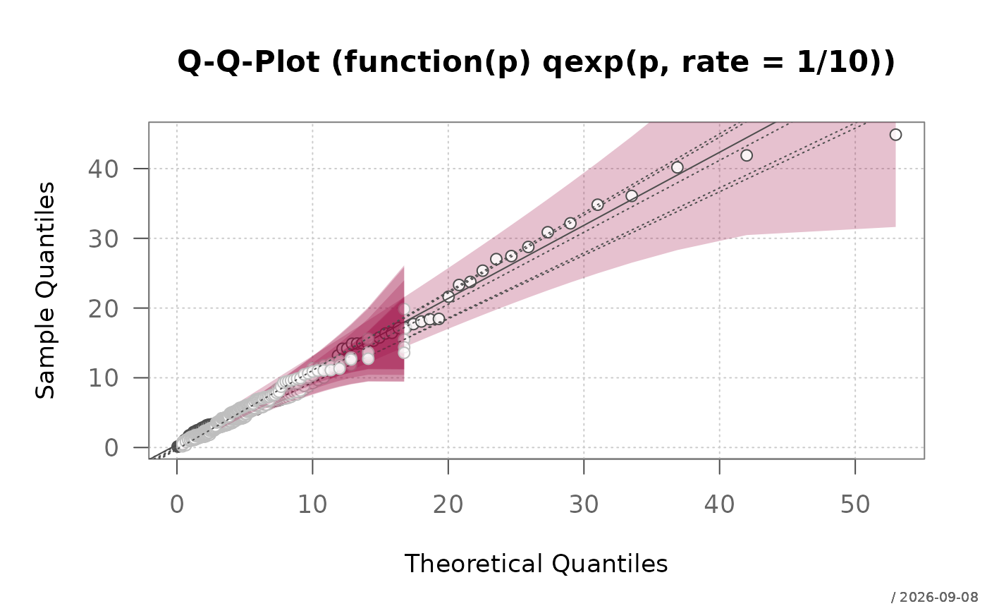
Create a QQ-plot for a variable of any distribution. The assumed underlying distribution can be defined as a function of f(p), including all required parameters. Confidence bands are provided by default.

Usage

plotQQ(
  x,
  qdist = stats::qnorm,
  main = NULL,
  xlab = NULL,
  ylab = NULL,
  datax = FALSE,
  add = FALSE,
  grid = .useTheme,
  box = .useTheme,
  cband = list(conf.level = 0.95),
  qqline = TRUE,
  stamp = .useTheme,
  ...
)

Arguments

x: the data sample
qdist: the quantile function of the assumed distribution. Can either be given as simple function name or defined as own function using the required arguments. Default is qnorm(). See examples.
main: the main title for the plot. This will be "Q-Q-Plot" by default
xlab: the xlab for the plot
ylab: the ylab for the plot
datax: logical. Should data values be on the x-axis? Default is FALSE.
add: logical specifying if the points should be added to an already existing plot; defaults to FALSE.
grid: controls drawing of the background grid. .useTheme (default) follows the active theme (getTheme()$grid). TRUE/FALSE/NA, or a named list, as for graphics::grid().
box: controls drawing of the plot box. .useTheme (default) resolves to getTheme()$box. TRUE/FALSE/NA, or a named list, as for graphics::box().
cband: controls the confidence band. FALSE, NULL, or NA suppress it. A named list configures it; its conf.level element (default 0.95) controls the confidence level of the pointwise Kolmogorov-Smirnov-based band (conf.level is consumed before the band is drawn and never forwarded as a graphical parameter). Other list elements (e.g. col, border) configure the band's appearance.
qqline: arguments for the qqline. This will be estimated as a line through the 25\ procedure as qqline() does for normal distribution (instead of set it to abline(a = 0, b = 1)). The quantiles can however be overwritten by setting the argument probs to some user defined values. Also the method for calculating the quantiles can be defined (default is 7, see quantile()). The line defaults are set to col = par("fg"), lwd = par("lwd") and lty = par("lty"). No line will be plotted if args.qqline is set to NA.
stamp: controls the corner stamp. .useTheme (default) resolves to getTheme()$stamp. TRUE/FALSE/NULL, a string, or a named list of arguments for stamp() (e.g. list(text = "...", las = 2)).
...: the dots are passed to the plot function.

Details

The function generates a sequence of points between 0 and 1 and transforms those into quantiles by means of the defined assumed distribution.

Note

The code is inspired by the tip 10.22 "Creating other Quantile-Quantile plots" from R Cookbook and based on R-Core code from the function qqline. The calculation of confidence bands are rewritten based on an algorithm published in the package BoutrosLab.plotting.general.

Based on code by Ying Wu

References

Teetor, P. (2011) R Cookbook. O'Reilly, pp. 254-255.

Examples


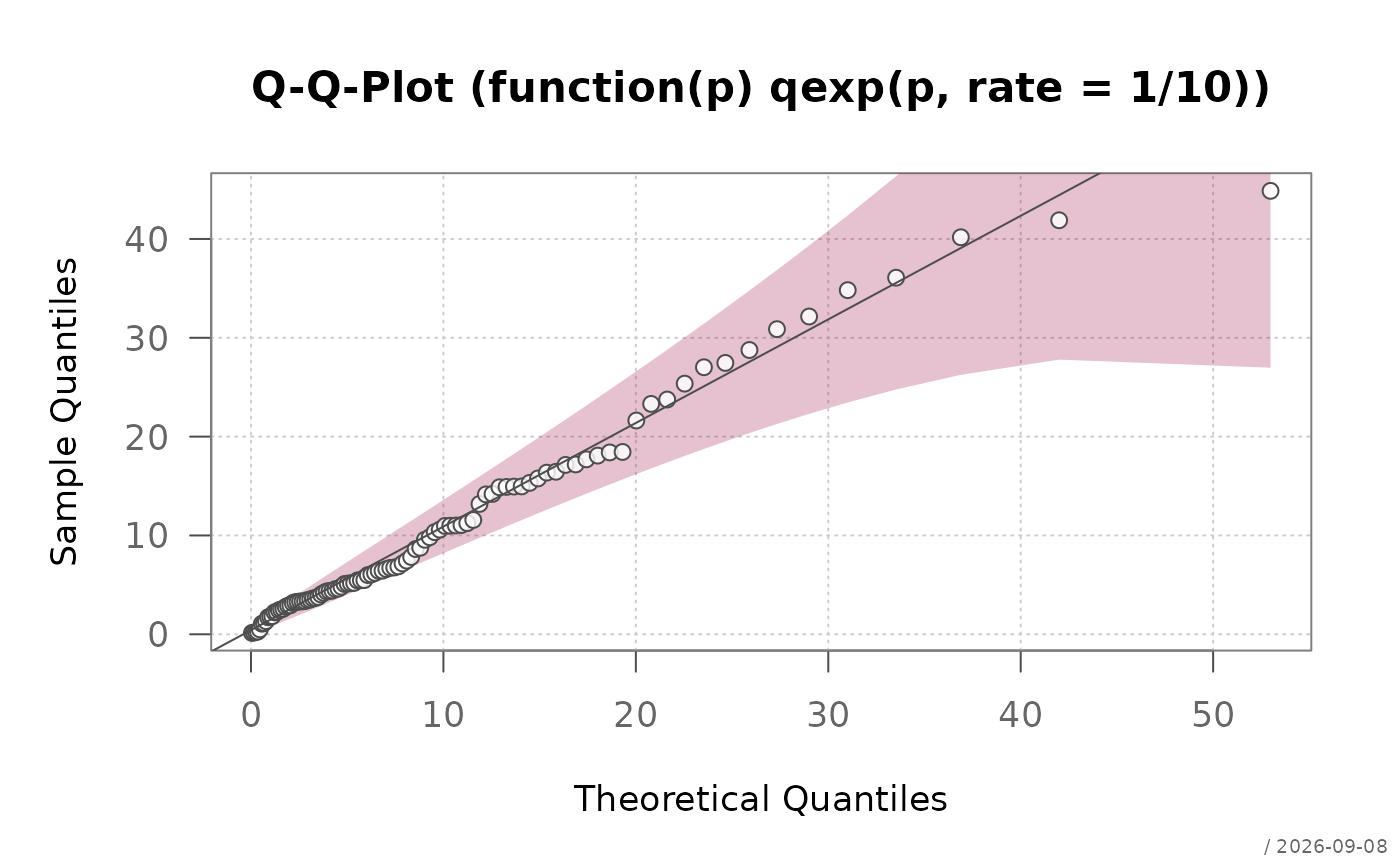
y <- rexp(100, 1/10)
plotQQ(y, function(p) qexp(p, rate=1/10))


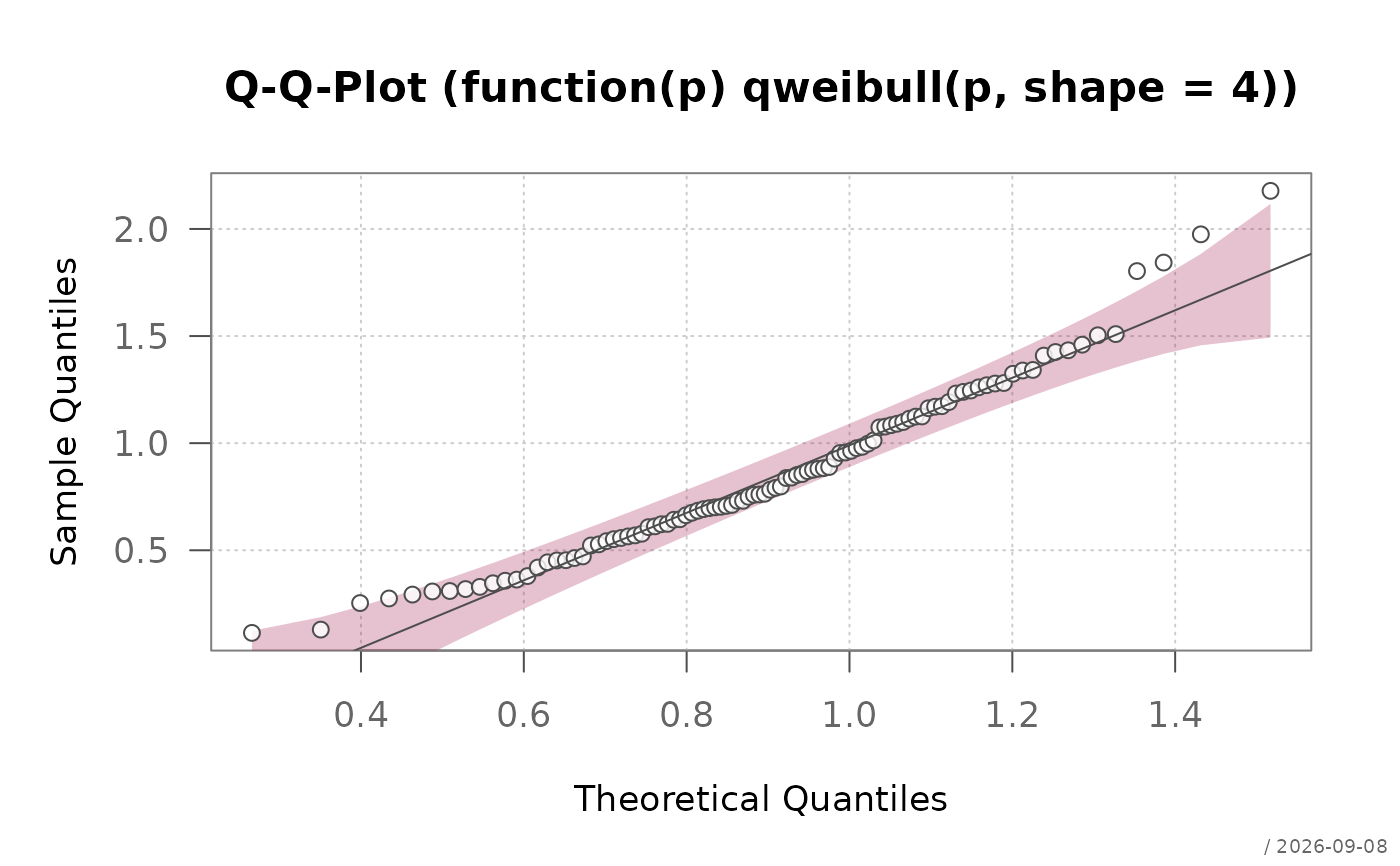
w <- rweibull(100, shape=2)
plotQQ(w, qdist = function(p) qweibull(p, shape=4))


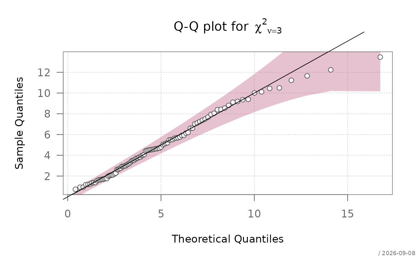
z <- rchisq(100, df=5)
plotQQ(z, function(p) qchisq(p, df=5),
       args.qqline=list(col=2, probs=c(0.1, 0.6)),
       main=expression("Q-Q plot for" ~~ {chi^2}[nu == 3]))
#> Warning: is.na() applied to non-(list or vector) of type 'expression'
#> Warning: "args.qqline" is not a graphical parameter
#> Warning: "args.qqline" is not a graphical parameter
#> Warning: "args.qqline" is not a graphical parameter
#> Warning: "args.qqline" is not a graphical parameter
#> Warning: "args.qqline" is not a graphical parameter
#> Warning: "args.qqline" is not a graphical parameter
abline(0,1)


# 90% confidence band instead of the 95% default
plotQQ(y, function(p) qexp(p, rate=1/10), cband = list(conf.level = 0.90))

# add 5 random sets
for(i in 1:5){
  z <- rchisq(100, df=5)
  plotQQ(z, function(p) qchisq(p, df=5), add=TRUE, args.qqline = NA,
         col="grey", lty="dotted")
}
#> Warning: "args.qqline" is not a graphical parameter
#> Warning: "args.qqline" is not a graphical parameter
#> Warning: "args.qqline" is not a graphical parameter
#> Warning: "args.qqline" is not a graphical parameter
#> Warning: "args.qqline" is not a graphical parameter