Frequency Distribution Plot

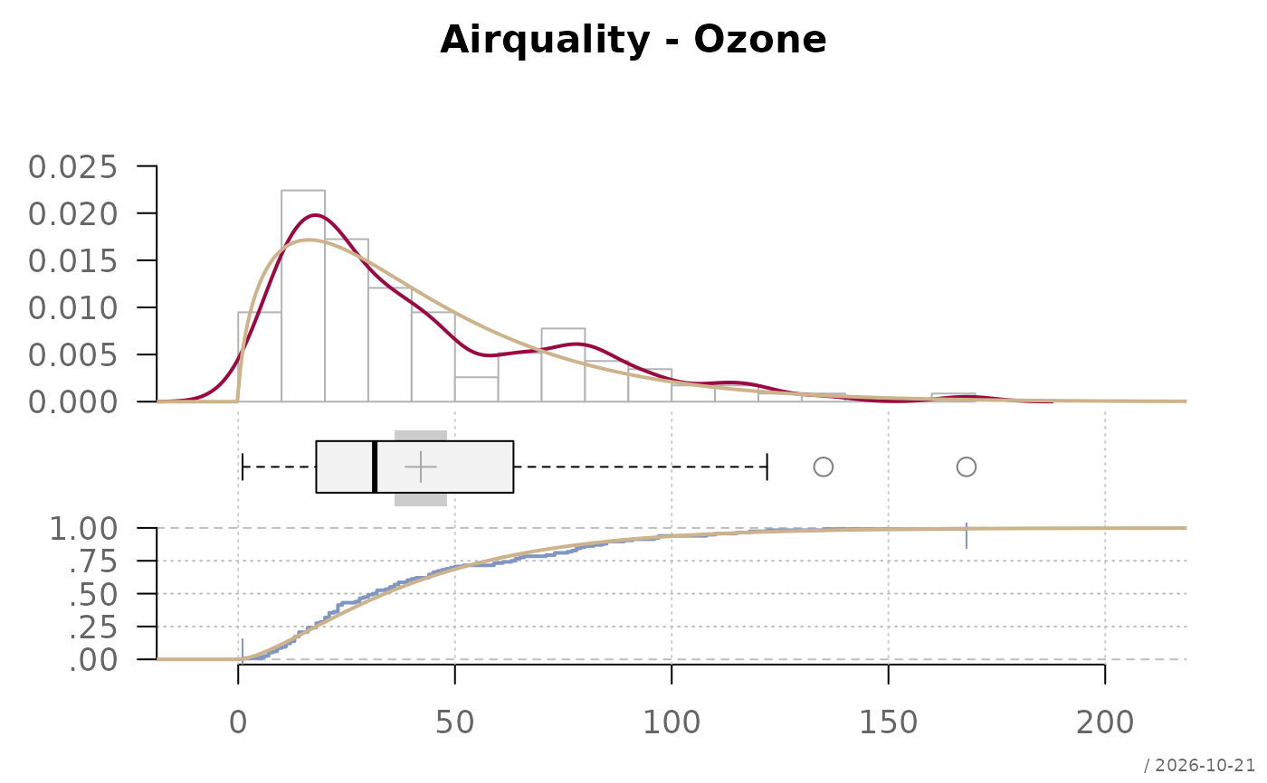
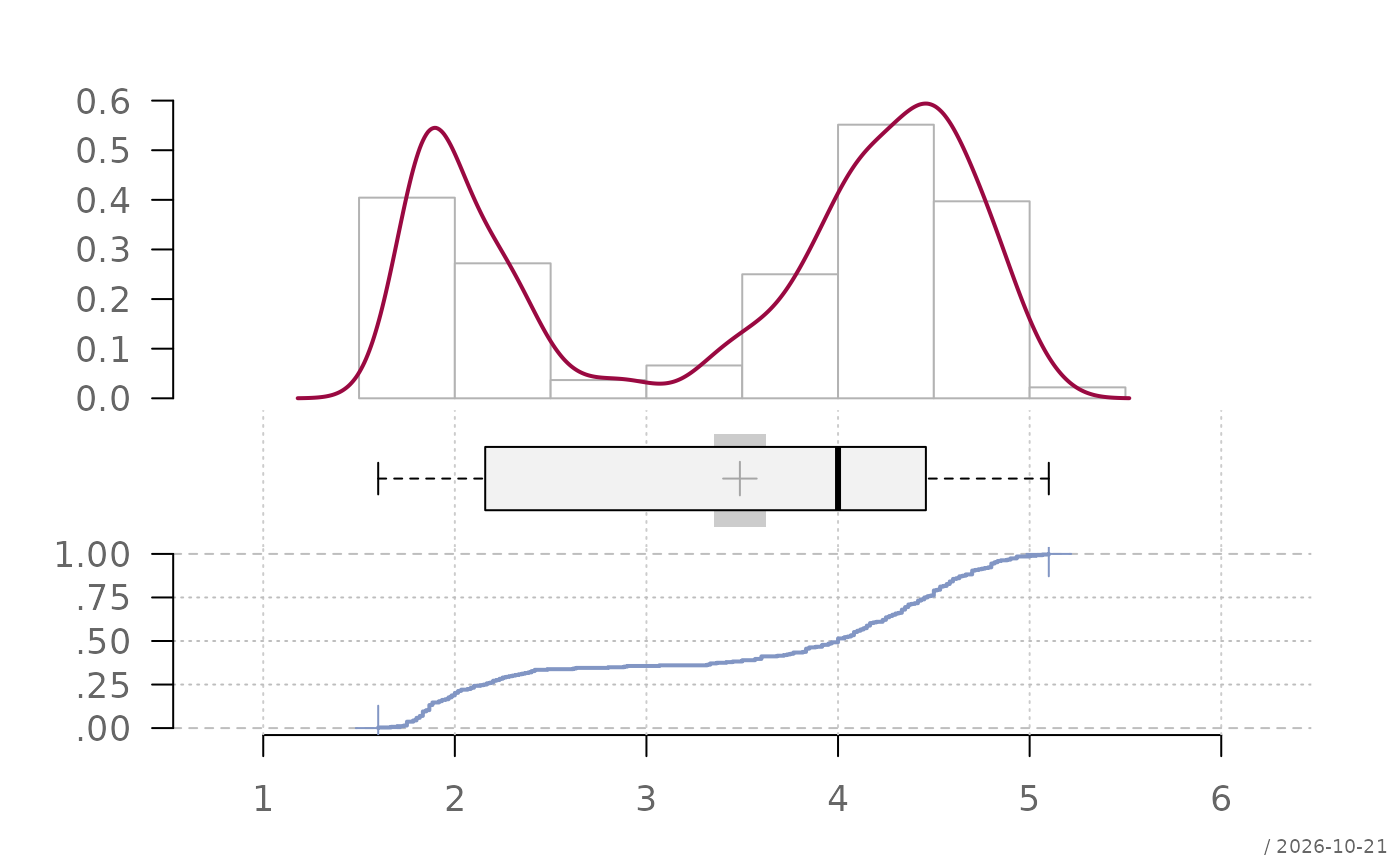
Creates a univariate graphical summary combining a histogram (or probability mass plot for discrete data), a kernel density curve, a boxplot, and an empirical cumulative distribution function in a single multi-panel figure. Optional components include a rug, and fitted theoretical distribution curves for both the histogram and the ECDF panel.

Usage

plotFreqDist(
  x,
  main = NULL,
  xlab = "",
  xlim = NULL,
  heights = NULL,
  hist = TRUE,
  dens = TRUE,
  rug = FALSE,
  curve = FALSE,
  boxplot = TRUE,
  ecdf = TRUE,
  curveEcdf = FALSE,
  stamp = .useTheme,
  ...
)

Arguments

x

numeric vector whose distribution is to be plotted.

main

main title. NULL (default) draws none, unless the theme sets autoTitle = TRUE (see theme); the title is then derived from the expression passed as x. "", NA or FALSE always suppress it and compact the top margin; any other string is used as given.

xlab

label for the x-axis. The variable name is typically placed in main, so this defaults to "".

xlim

range of the x-axis. NULL (default) uses a pretty range of the non-missing values in x.

heights

numeric vector of relative panel heights for layout(): three values for histogram/boxplot/ecdf, two for histogram/boxplot or histogram/ecdf only. NULL (default) chooses automatically.

hist

controls the histogram panel. TRUE (default) uses package defaults; FALSE/NA suppresses the panel (xlim then falls back to the pretty range of the data); a list overrides specific arguments forwarded to graphics::hist(). The element type selects the plot style: "hist" (standard histogram, chosen automatically for continuous or high-cardinality data) or "mass" (vertical bars per unique value, for discrete/low-cardinality data). The element panel.last adds to the histogram after it is drawn: a function without arguments or a quoted call, e.g. list(panel.last = quote(abline(v = 0, lty = 2))).

dens

controls the kernel density curve. TRUE (default) draws a curve via stats::density(); a list overrides specific arguments (e.g. list(bw = 0.1, col = "red")).

rug

controls a rug plot. FALSE (default) suppresses it; TRUE or a list draw a rug via graphics::rug().

curve

controls a fitted theoretical distribution curve on the histogram. FALSE (default), NULL, or NA suppress it; TRUE draws a normal curve with mean(x)/sd(x); a list may include expr as a function of x or a one-sided formula in x for any distribution (e.g. list(expr = ~ dt(x, df = 2), col = "darkgreen")). The formula is evaluated in the environment it was written in, so local variables may be referenced (see the gamma example below).

boxplot

controls the boxplot panel. TRUE (default) draws a horizontal boxplot with a mean marker and CI band; FALSE/ NA suppresses the panel. A list overrides arguments forwarded to graphics::boxplot(); two extra elements control the mean display: pch.mean (default 3) and col.meanci (default getTheme()$grid$col). Set either to NA to suppress that element.

ecdf

controls the ECDF panel. TRUE (default) calls plotECDF(); a list overrides specific arguments.

curveEcdf

controls a fitted theoretical CDF curve on the ECDF panel, analogous to curve. FALSE (default) suppresses it.

stamp

controls the corner stamp. .useTheme (default) resolves to getTheme()$stamp. TRUE/FALSE/ NULL, a string, or a named list for stamp().

...

further graphical parameters passed to par() via the internal framework. Note that mar given here sets the outer margins (oma) of the multi-panel figure; the inner panel margins are managed internally and cannot be overridden.

Value

No return value (invisible NULL), called for its side effect of drawing the plot.

Details

Each plot component is controlled via a single argument accepting bedrock::callIf() semantics:

• TRUE: draw with package defaults

• FALSE, NULL, or NA: suppress entirely

• a named list: draw with the given overrides merged into the defaults

Performance: for very large vectors (n > 1e7) the density curve, ECDF, and semi-transparent boxplot outliers will still take noticeable time. For exploratory work on very large data, consider sampling first: plotFreqDist(x[sample(length(x), 5000)]).

See also

hist(), boxplot(), plotECDF(), density(), rug(), layout(), theme

Other plot.univariate: plotArea(), plotBar(), plotBox(), plotCatDist(), plotDens(), plotDensBox(), plotDot(), plotECDF(), plotLines(), plotQQ(), plotViolin()

Examples

plotFreqDist(faithful$eruptions)


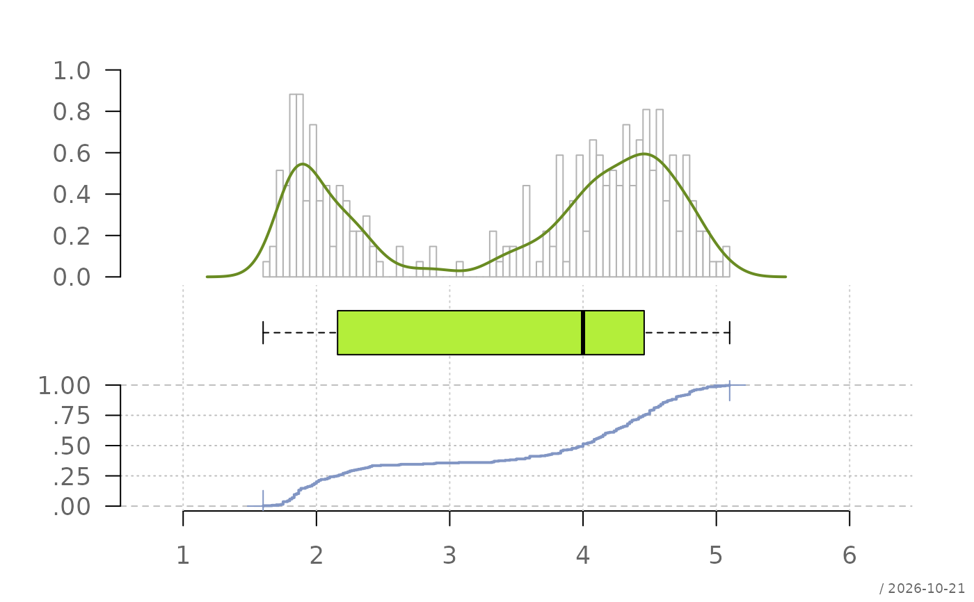
# custom histogram breaks, density color, boxplot styling
plotFreqDist(faithful$eruptions,
  hist    = list(breaks = 50),
  dens    = list(col = "olivedrab4"),
  boxplot = list(col = "olivedrab2", pch.mean = NA, col.meanci = NA))


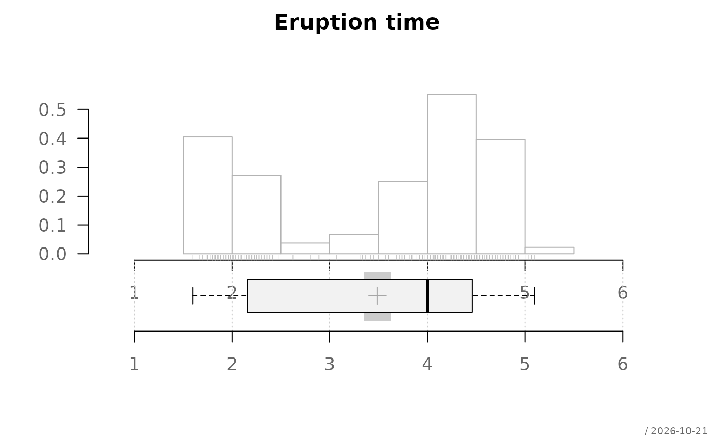
# no density, no ecdf, add rug instead
plotFreqDist(faithful$eruptions,
  dens = FALSE, ecdf = FALSE,
  hist = list(xaxt = "s"),
  rug  = TRUE,
  heights = c(3, 2.5), 
  main = "Eruption time")


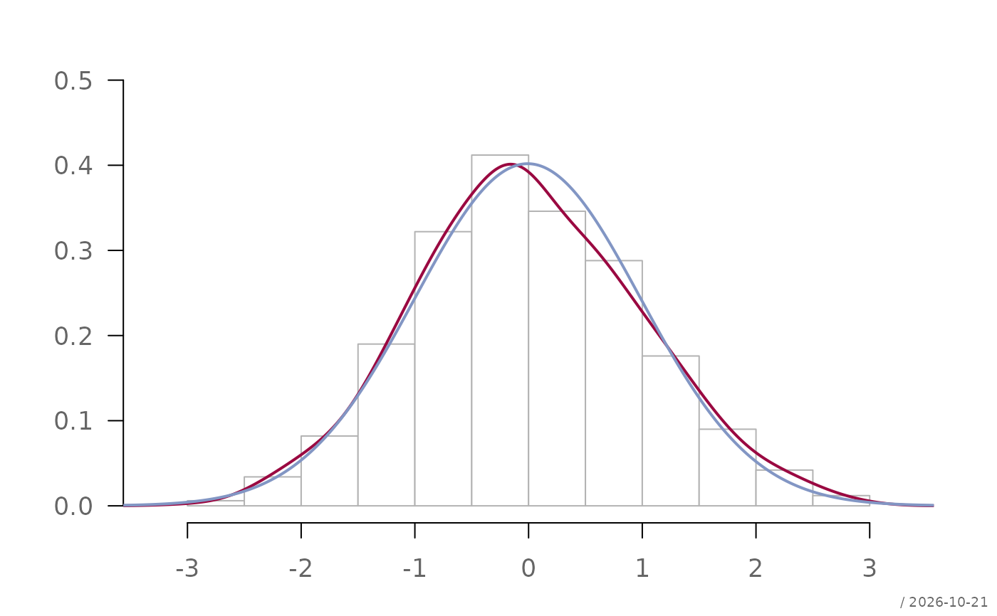
# overlay a normal density curve
x <- rnorm(1000)
plotFreqDist(x, curve = TRUE, boxplot = FALSE, ecdf = FALSE)


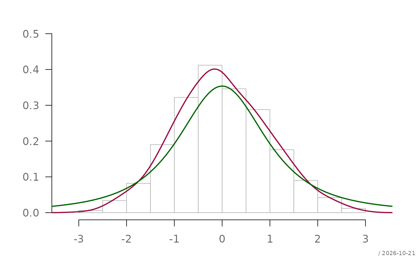
# compare with a t-distribution curve
plotFreqDist(x,
  curve   = list(expr = ~ dt(x, df = 2), col = "darkgreen"),
  boxplot = FALSE, ecdf = FALSE)


# overlay gamma distribution on both histogram and ECDF
ozone <- airquality$Ozone
m <- mean(ozone, na.rm = TRUE)
v <- var(ozone, na.rm = TRUE)
plotFreqDist(ozone,
  hist       = list(breaks = 15),
  curve      = list(expr = ~ dgamma(x, shape = m^2/v, scale = v/m),
                    col = "navajowhite3"),
  curveEcdf  = list(expr = ~ pgamma(x, shape = m^2/v, scale = v/m),
                    col = "navajowhite3"),
  main = "Airquality - Ozone")