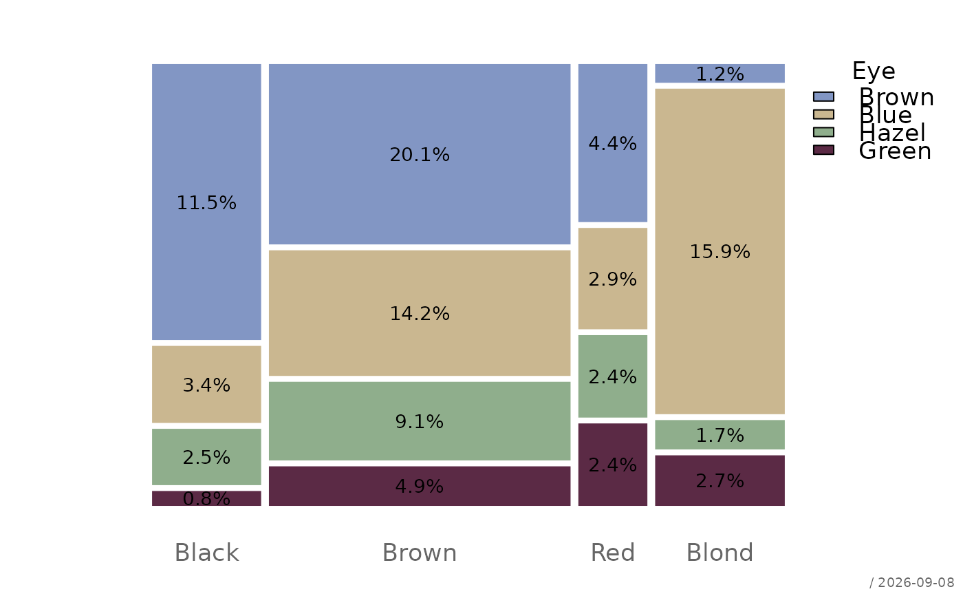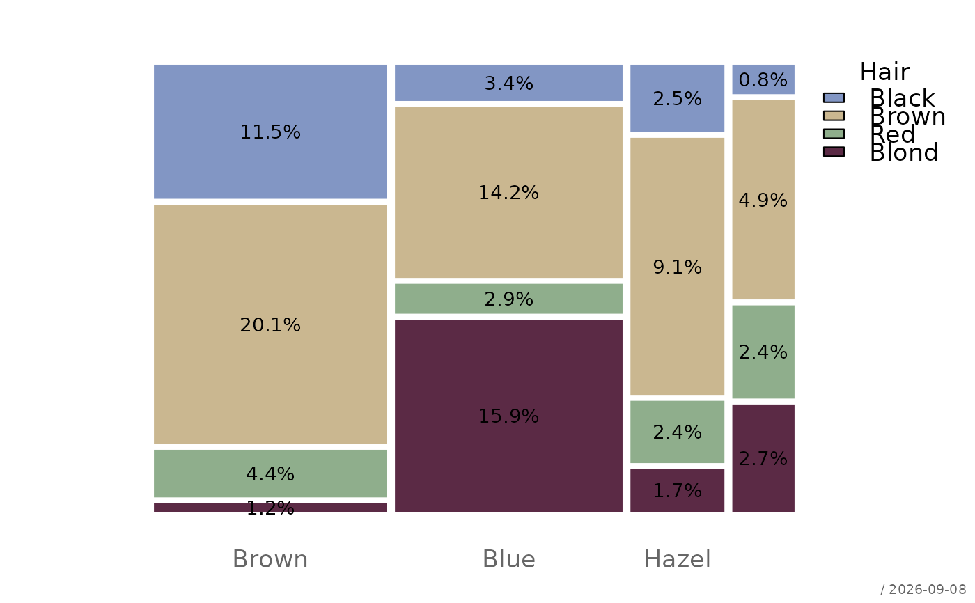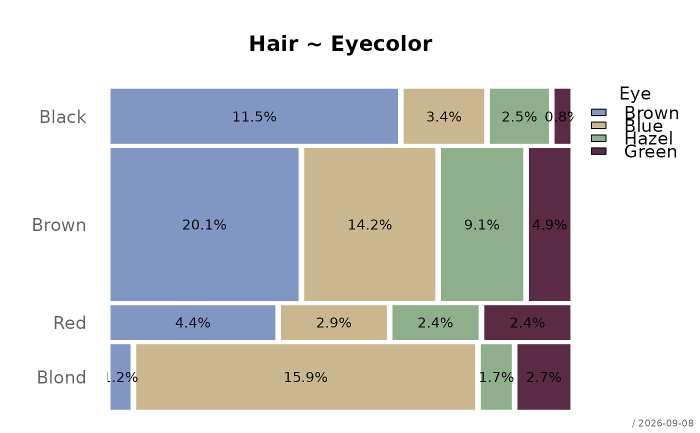
Mosaic Plot for 2-Way Contingency Tables

Draws a mosaic plot (spine plot) for a 2-way contingency table, with proportional tile areas, optional cell labels (counts or percentages), and a "Few"-style minimal appearance (white tile separators, muted palette, optional legend).

Usage

plotMosaic(
  x,
  main = "",
  xlab = NULL,
  ylab = NULL,
  swap = FALSE,
  horiz = FALSE,
  gap = 0.01,
  col = .useTheme,
  border = "white",
  legend = TRUE,
  labels = c("p", "n", "none"),
  labCex = 0.8,
  labDigits = 1,
  stamp = .useTheme,
  ...
)

Arguments

x: a 2-way contingency table, matrix, or array coercible via as.table(). Higher-dimensional arrays must be collapsed first, e.g. via apply(x, c(1,2), sum).
main: character. Plot title. Default "" (no title).
xlab, ylab: character or NULL. Axis labels. Default NULL (no labels), since the category levels together with main and the legend title are usually self-explanatory.
swap: logical. If TRUE, transpose the two dimensions of x before plotting, so the second table dimension determines the x-axis split and the first becomes the fill/legend variable. Default FALSE.
horiz: logical. If TRUE, draw the mosaic horizontally: the first table dimension is shown top-to-bottom on the y-axis instead of left-to-right on the x-axis. Default FALSE.
gap: numeric. Width of the white separator drawn between adjacent tiles, in plot-region units ([0, 1]). Default 0.01.
col: vector of colors for the fill/legend variable (the second table dimension, or first if swap = TRUE). .useTheme (default) resolves to pal(getTheme()$palette, n = <number of levels>) - the active theme's qualitative palette (see theme), sampled or interpolated to match the number of category levels. A diverging or sequential color ramp is deliberately not used here: the fill variable is an unordered categorical variable, and a ramp would visually suggest an ordering between levels that doesn't exist.
border: color of the tile borders. Default "white".
legend: logical. Draw a legend for the fill variable. Default TRUE.
labels: character, one of "p", "n", "none". Cell labels showing the proportion of the table total ("p"), the absolute frequency ("n"), or no labels ("none"). Labels are only drawn for tiles large enough to hold them. Default "p".
labCex: numeric. Character expansion factor for cell labels. Default 0.8.
labDigits: integer. Number of decimal digits for percentage cell labels when labels = "p". Default 1.
stamp: controls the corner stamp. .useTheme (default) resolves to getTheme()$stamp. TRUE/FALSE/ NULL, or an explicit string, as for .withGraphicsState() (internal).
...: further graphical parameters passed to par() via .applyParFromDots(), e.g. mar, cex.axis, las.

Value

Invisibly, the data.frame of tile geometry as produced by .computeMosaicTiles(), with columns x0, x1, y0, y1, n, p, pCond and one column per table dimension. This allows users to add further annotations (e.g. via rect() or text()) on top of the plot.

Details

Cells belonging to a row with a row total of zero are drawn as zero-height tiles and receive no label, but do not cause an error or NaN in the geometry.

In both orientations only the first table dimension receives an axis (its split points are constant across the whole plot); the second dimension's split points vary per column/row and are represented via the legend only. No numeric probability axis is drawn. The second dimension is stacked top-down (vertical) resp. left-to-right (horiz = TRUE): its first level sits at the top / left, matching graphics::spineplot() and the legend order.

Examples

tab <- apply(HairEyeColor, c(1, 2), sum)

plotMosaic(tab)

plotMosaic(tab, swap = TRUE)

plotMosaic(tab, horiz = TRUE, main = "Hair ~ Eyecolor")