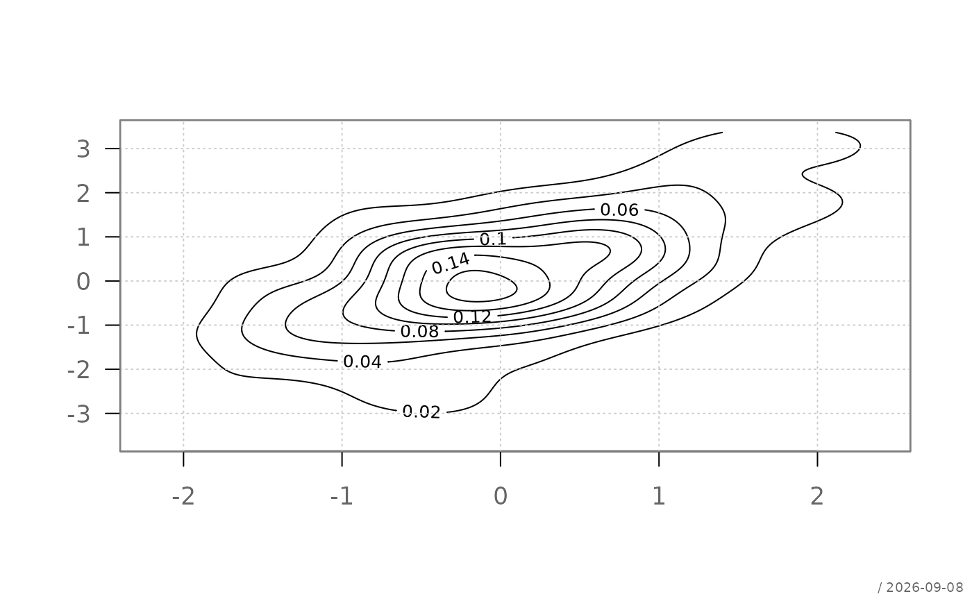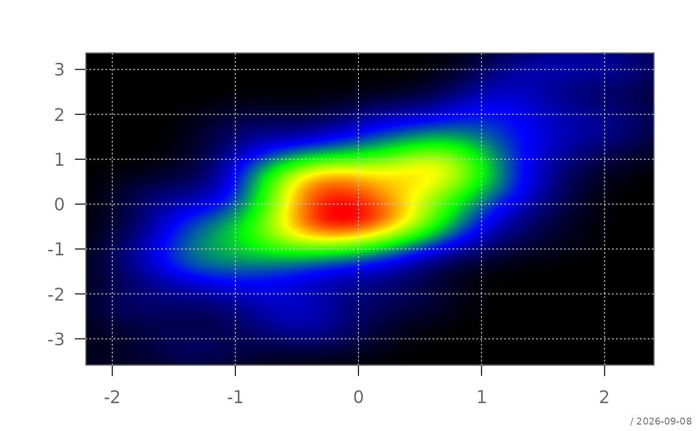
Computes a two-dimensional kernel density estimate and visualises it using contour, image, or perspective plots.
Arguments
- x
numeric vector of x-coordinates.
- y
numeric vector of y-coordinates. Must have the same length as
x.- main
optional main title of the plot.
- xlab, ylab
axis labels.
- xlim, ylim
numeric vectors of length two specifying axis limits.
- type
character string specifying the plot type. One of
"contour","image", or"persp".- col
color specification used for
type = "image". Defaults to a reversed"red-black"sequential ramp (pal()), running from black (low density) to red (high density) - hardcoded rather than theme-driven, since this is a continuous, unidirectional gradient, unlike the active theme's categoricalpaletteor divergingtwinpair, neither of which fits a density surface.- grid
controls drawing of the background grid.
.useTheme(default) follows the active theme (getTheme()$grid).TRUE/FALSE/NA, or a named list, as forgraphics::grid().- box
controls drawing of the plot box.
.useTheme(default) resolves togetTheme()$box.TRUE/FALSE/NA, or a named list, as forgraphics::box().- stamp
controls the corner stamp.
.useTheme(default) resolves togetTheme()$stamp.TRUE/FALSE/NULL, a string, or a named list forstamp().- ...
additional graphical parameters passed to underlying plotting functions.
Value
Invisibly returns the result of the selected plotting call. Typically a list containing grid coordinates and estimated density values.
Details
The function estimates a bivariate density surface using a Gaussian kernel with bandwidths determined via a normal reference rule. The density is evaluated on a regular grid and visualised using one of three base graphics representations:
"contour": contour lines of equal density"image": raster representation of the density surface"persp": three-dimensional perspective plot
The choice of representation affects interpretability: contour and image plots emphasise structure in the data distribution, while perspective plots highlight global shape but may distort local density.
Bandwidth selection follows a rule-of-thumb approach based on spread (interquartile range and variance), which provides a reasonable default for unimodal distributions but may oversmooth multimodal structures.
Missing or non-finite values are not allowed and will result in an error.
See also
Other plot.bivariate:
plotAssoc(),
plotBag(),
plotCor(),
plotHeatmap(),
plotHexbin(),
plotMosaic(),
plotXY()