Computes and displays a comprehensive set of descriptive statistics and
association measures for a contingency table (r x c or 2 x 2). The function
is also dispatched for matrix and cross-classified factor pairs via
Desc.qq and Desc.matrix.
Usage
# S3 method for class 'table'
desc(
  x,
  conf.level = 0.95,
  prop = NULL,
  main = NULL,
  verbose = NULL,
  plotit = NULL,
  ...
)

# S3 method for class 'matrix'
desc(
  x,
  conf.level = 0.95,
  prop = NULL,
  main = NULL,
  verbose = NULL,
  plotit = NULL,
  ...
)

# S3 method for class 'array'
desc(
  x,
  conf.level = 0.95,
  prop = NULL,
  main = NULL,
  verbose = NULL,
  plotit = NULL,
  ...
)

# S3 method for class 'Desc.table'
print(x, printHeader = TRUE, ...)
Arguments
- x
a
tableormatrixobject. For the formula interface, usedesc(y ~ x, data)which dispatches to this function automatically.- conf.level
numeric, confidence level for all confidence intervals. Default is
0.95.- prop
character string controlling which proportions are shown in the cross-tabulation. One of
"rows","cols","total", or"no"(frequencies only). IfNULL(default),"rows"is used, and all three proportions atverbose = 3; an explicit value is always respected.- main
main title for the plot
- verbose
integer controlling the amount of output (1, 2, or 3).
NULL(default) falls back togetOption("DescTools.verbose", 2). If set explicitly in the function call, that value takes priority over the global option. See Details for what each level produces.- plotit
whether a plot is produced automatically
- ...
further arguments passed to or from other methods
- printHeader
whether the header is printed
Value
an object of class c("Desc.table", "Desc").
The object is a list containing all computed statistics and is intended
to be used via its print and plot methods.
Details
The verbose argument controls which statistics are displayed. All
of them are computed in any case; the lists below describe the printed
output. The cross-tabulation always shows the frequencies together with
the proportions selected by prop.
2 x 2 tables
verbose = 1: chi-squared test with Yates continuity correction, Fisher's exact testverbose = 2(default): additionally McNemar's test and a table of odds ratio, relative risks (col1, col2) and proportion difference, each with confidence intervalverbose = 3: additionally the uncorrected Pearson chi-squared test, and relative risks (row1, row2), Cramér's V and Cohen's h in the table of estimates
r x c tables
verbose = 1: Pearson chi-squared testverbose = 2(default): additionally the G-test (log likelihood ratio) and the Mantel-Haenszel chi-squared test, and the point estimates of the first three association measuresverbose = 3: the full table of nominal and ordinal association measures with confidence intervals (Cramér's V, contingency coefficient, lambda, uncertainty coefficient, mutual information, gamma, tau-b, tau-c, Somers' D, Pearson and Spearman correlation)
Table types:
For r x c tables (arbitrary number of rows and columns) all nominal and ordinal association measures listed above are available. For 2 x 2 tables the output additionally includes tests and measures specific to the 2 x 2 case (Fisher's exact, McNemar, odds ratio, relative risk, proportions difference).
Dispatching:
desc.matrix and desc.qq both redirect to desc.table.
When called via the formula interface desc(y ~ x, data), the type
of y and x is known and ordinal-specific measures
(tau-b and above) are activated automatically when both variables are
ordered factors.
Plots
The plot method pharos::plot.Desc.table() is part of pharos; its help
page documents which and all further arguments. The displays are
drawn by pharos::plotMosaic(), pharos::plotAssoc() and
pharos::plotHeatmap(), among others.
See also
desc() for the generic function and formula interface,
desc.qq() for categorical ~ categorical via the formula interface,
desc.numeric() for univariate numeric descriptions,
desc.factor() for univariate factor descriptions,
stats::chisq.test(), stats::fisher.test(),
cramerV(), oddsRatio()
Plot method: pharos::plot.Desc.table()
Other desc:
desc(),
desc.Date(),
desc.factor(),
desc.nn,
desc.nq,
desc.numeric(),
desc.qn,
desc.qq,
desc.ts()
Examples
# from an existing table
tab <- table(Pizza$driver, Pizza$area)
desc(tab)
#> ──────────────────────────────────────────────────────────────────────────────
#> tab (table)
#>
#> Summary:
#> n: 1194, rows: 7, columns: 3
#>
#> Brent Camden Westminster Sum
#>
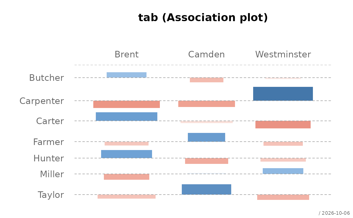
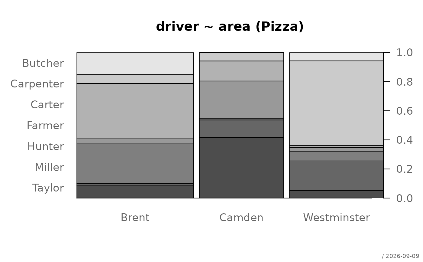
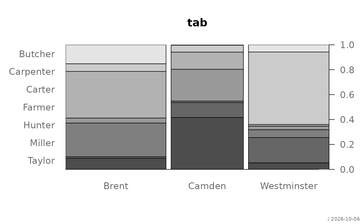
#> Butcher freq 72 1 22 95
#> p.row 75.8% 1.1% 23.2% 8.0%
#>
#> Carpenter freq 29 19 221 269
#> p.row 10.8% 7.1% 82.2% 22.5%
#>
#> Carter freq 177 47 5 229
#> p.row 77.3% 20.5% 2.2% 19.2%
#>
#> Farmer freq 19 87 11 117
#> p.row 16.2% 74.4% 9.4% 9.8%
#>
#> Hunter freq 128 4 24 156
#> p.row 82.1% 2.6% 15.4% 13.1%
#>
#> Miller freq 6 41 77 124
#> p.row 4.8% 33.1% 62.1% 10.4%
#>
#> Taylor freq 42 142 20 204
#> p.row 20.6% 69.6% 9.8% 17.1%
#>
#> Sum freq 473 341 380 1194
#> p.row 39.6% 28.6% 31.8% 100.0%
#>
#>
#> Pearson's Chi-squared test:
#> X-squared = 1009.5, df = 12, p-value < 2.2e-16
#> Log likelihood ratio (G-test) test of independence:
#> G = 1020.9, df = 12, p-value < 2.2e-16
#> Mantel-Haenszel Chi-squared:
#> X-squared = 2.6144, df = 1, p-value = 0.1059
#>
#> Contingency Coeff. 0.677
#> Cramer V 0.650
#> Kendall Tau-b -0.057
#>
 desc(tab, prop = "rows", verbose = 3)
#> ──────────────────────────────────────────────────────────────────────────────
#> tab (table)
#>
#> Summary:
#> n: 1194, rows: 7, columns: 3
#>
#> Brent Camden Westminster Sum
#>
#> Butcher freq 72 1 22 95
#> p.row 75.8% 1.1% 23.2% 8.0%
#>
#> Carpenter freq 29 19 221 269
#> p.row 10.8% 7.1% 82.2% 22.5%
#>
#> Carter freq 177 47 5 229
#> p.row 77.3% 20.5% 2.2% 19.2%
#>
#> Farmer freq 19 87 11 117
#> p.row 16.2% 74.4% 9.4% 9.8%
#>
#> Hunter freq 128 4 24 156
#> p.row 82.1% 2.6% 15.4% 13.1%
#>
#> Miller freq 6 41 77 124
#> p.row 4.8% 33.1% 62.1% 10.4%
#>
#> Taylor freq 42 142 20 204
#> p.row 20.6% 69.6% 9.8% 17.1%
#>
#> Sum freq 473 341 380 1194
#> p.row 39.6% 28.6% 31.8% 100.0%
#>
#>
#> Pearson's Chi-squared test:
#> X-squared = 1009.5, df = 12, p-value < 2.2e-16
#> Log likelihood ratio (G-test) test of independence:
#> G = 1020.9, df = 12, p-value < 2.2e-16
#> Mantel-Haenszel Chi-squared:
#> X-squared = 2.6144, df = 1, p-value = 0.1059
#>
#> est lci uci
#> Contingency Coeff. 0.677 0.658 0.696
#> Cramer V 0.650 0.606 0.687
#> Kendall Tau-b -0.057 -0.107 -0.008
#> Goodman Kruskal Gamma -0.071 -0.132 -0.010
#> Stuart Tau-c -0.064 -0.119 -0.009
#> Somers D R|C -0.065 -0.120 -0.009
#> Pearson Correlation -0.047 -0.103 0.010
#> Spearman Correlation -0.075 -0.131 -0.019
#> Lambda R|C 0.293 0.259 0.327
#> Lambda sym 0.426 0.393 0.460
#> Uncertainty Coeff. R|C 0.227 0.204 0.250
#> Uncertainty Coeff. sym 0.288 0.259 0.316
#> Mutual Information 0.617 - -
#>
#> ────────────────────
#> ¹ 95% conf. level
#>
desc(tab, prop = "rows", verbose = 3)
#> ──────────────────────────────────────────────────────────────────────────────
#> tab (table)
#>
#> Summary:
#> n: 1194, rows: 7, columns: 3
#>
#> Brent Camden Westminster Sum
#>
#> Butcher freq 72 1 22 95
#> p.row 75.8% 1.1% 23.2% 8.0%
#>
#> Carpenter freq 29 19 221 269
#> p.row 10.8% 7.1% 82.2% 22.5%
#>
#> Carter freq 177 47 5 229
#> p.row 77.3% 20.5% 2.2% 19.2%
#>
#> Farmer freq 19 87 11 117
#> p.row 16.2% 74.4% 9.4% 9.8%
#>
#> Hunter freq 128 4 24 156
#> p.row 82.1% 2.6% 15.4% 13.1%
#>
#> Miller freq 6 41 77 124
#> p.row 4.8% 33.1% 62.1% 10.4%
#>
#> Taylor freq 42 142 20 204
#> p.row 20.6% 69.6% 9.8% 17.1%
#>
#> Sum freq 473 341 380 1194
#> p.row 39.6% 28.6% 31.8% 100.0%
#>
#>
#> Pearson's Chi-squared test:
#> X-squared = 1009.5, df = 12, p-value < 2.2e-16
#> Log likelihood ratio (G-test) test of independence:
#> G = 1020.9, df = 12, p-value < 2.2e-16
#> Mantel-Haenszel Chi-squared:
#> X-squared = 2.6144, df = 1, p-value = 0.1059
#>
#> est lci uci
#> Contingency Coeff. 0.677 0.658 0.696
#> Cramer V 0.650 0.606 0.687
#> Kendall Tau-b -0.057 -0.107 -0.008
#> Goodman Kruskal Gamma -0.071 -0.132 -0.010
#> Stuart Tau-c -0.064 -0.119 -0.009
#> Somers D R|C -0.065 -0.120 -0.009
#> Pearson Correlation -0.047 -0.103 0.010
#> Spearman Correlation -0.075 -0.131 -0.019
#> Lambda R|C 0.293 0.259 0.327
#> Lambda sym 0.426 0.393 0.460
#> Uncertainty Coeff. R|C 0.227 0.204 0.250
#> Uncertainty Coeff. sym 0.288 0.259 0.316
#> Mutual Information 0.617 - -
#>
#> ────────────────────
#> ¹ 95% conf. level
#>
 # 2x2 table — additional measures are shown automatically
tab2 <- tab[1:2, 1:2]
desc(tab2)
#> ──────────────────────────────────────────────────────────────────────────────
#> tab2 (table)
#>
#> Summary:
#> n: 121, rows: 2, columns: 2
#>
#> Brent Camden Sum
#>
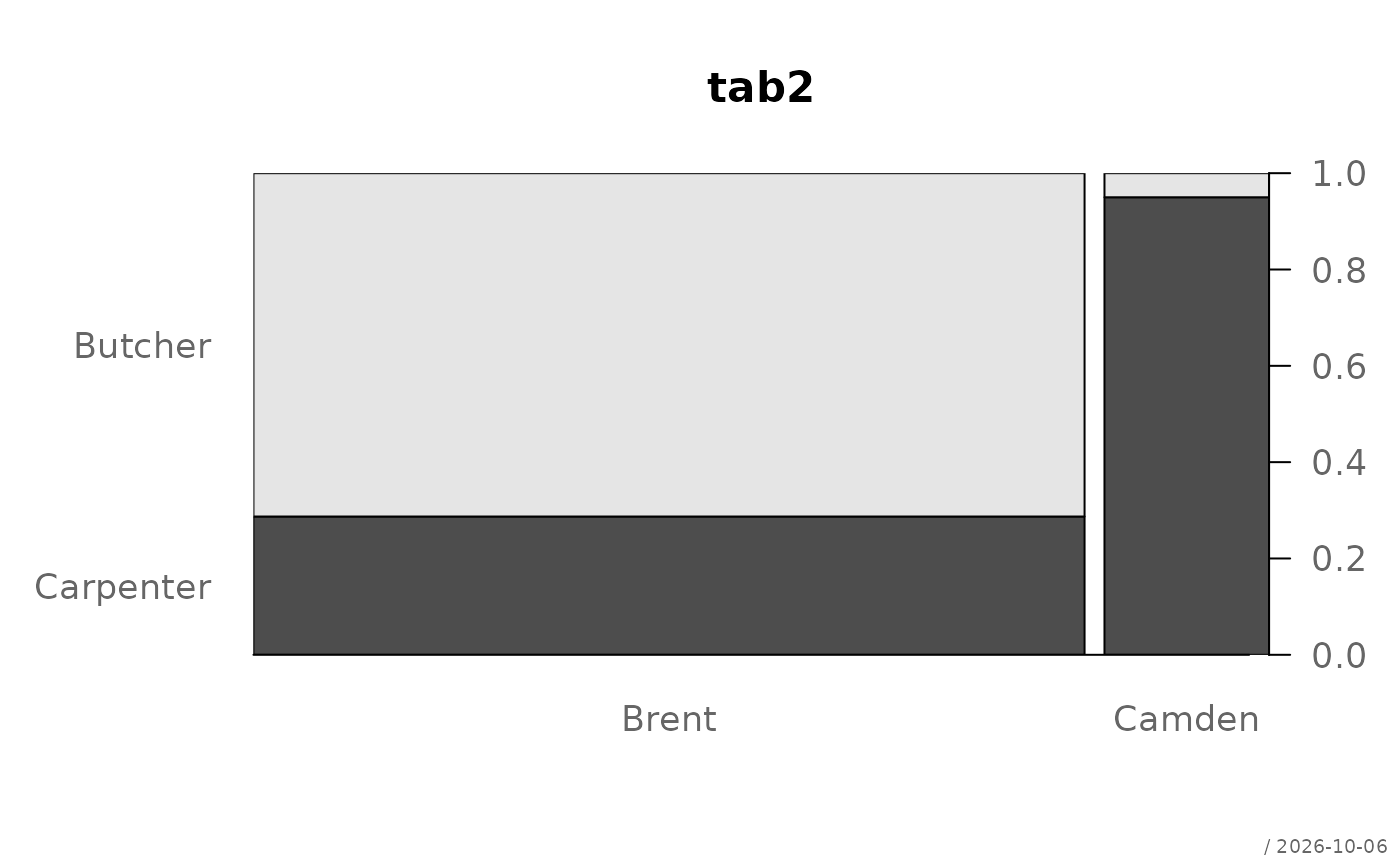
#> Butcher freq 72 1 73
#> p.row 98.6% 1.4% 60.3%
#>
#> Carpenter freq 29 19 48
#> p.row 60.4% 39.6% 39.7%
#>
#> Sum freq 101 20 121
#> p.row 83.5% 16.5% 100.0%
#>
#>
#> Pearson's Chi-squared test (cont. adj):
#> X-squared = 27.943, df = 1, p-value = 1.249e-07
#> Fisher's exact test p-value = 2.435e-08
#> McNemar's chi-squared = 24.3, df = 1, p-value = 8.244e-07
#>
#> est lci uci¹
#>
#> odds ratio 47.172 6.033 368.844
#> rel. risk (col1) 1.632 1.296 2.056
#> rel. risk (col2) 0.035 0.005 0.250
#> prop. diff 0.382 0.251 0.526
#>
#> ────────────────────
#> ¹ 95% conf. level
#>
# 2x2 table — additional measures are shown automatically
tab2 <- tab[1:2, 1:2]
desc(tab2)
#> ──────────────────────────────────────────────────────────────────────────────
#> tab2 (table)
#>
#> Summary:
#> n: 121, rows: 2, columns: 2
#>
#> Brent Camden Sum
#>
#> Butcher freq 72 1 73
#> p.row 98.6% 1.4% 60.3%
#>
#> Carpenter freq 29 19 48
#> p.row 60.4% 39.6% 39.7%
#>
#> Sum freq 101 20 121
#> p.row 83.5% 16.5% 100.0%
#>
#>
#> Pearson's Chi-squared test (cont. adj):
#> X-squared = 27.943, df = 1, p-value = 1.249e-07
#> Fisher's exact test p-value = 2.435e-08
#> McNemar's chi-squared = 24.3, df = 1, p-value = 8.244e-07
#>
#> est lci uci¹
#>
#> odds ratio 47.172 6.033 368.844
#> rel. risk (col1) 1.632 1.296 2.056
#> rel. risk (col2) 0.035 0.005 0.250
#> prop. diff 0.382 0.251 0.526
#>
#> ────────────────────
#> ¹ 95% conf. level
#>
 # formula interface — dispatches to desc.table internally
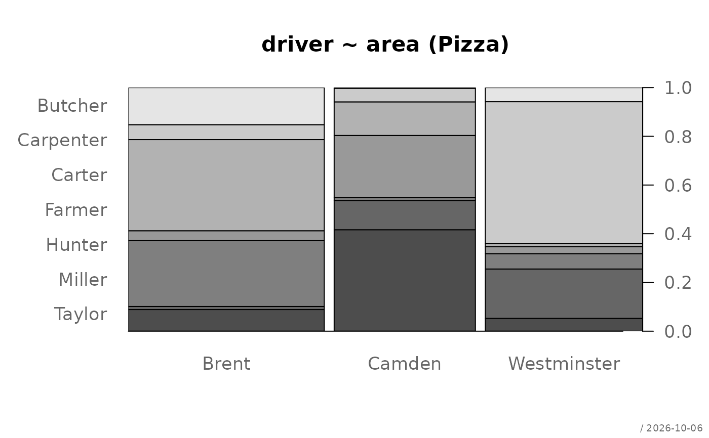
desc(driver ~ area, data = Pizza)
#> ──────────────────────────────────────────────────────────────────────────────
#> driver ~ area (Pizza) (Desc.qq)
#>
#> Summary:
#> pairs: 1209, valid: 1194 (98.8%), missings: 15 (1.2%)
#>
#> Brent Camden Westminster Sum
#>
#> Butcher freq 72 1 22 95
#> p.row 75.8% 1.1% 23.2% 8.0%
#>
#> Carpenter freq 29 19 221 269
#> p.row 10.8% 7.1% 82.2% 22.5%
#>
#> Carter freq 177 47 5 229
#> p.row 77.3% 20.5% 2.2% 19.2%
#>
#> Farmer freq 19 87 11 117
#> p.row 16.2% 74.4% 9.4% 9.8%
#>
#> Hunter freq 128 4 24 156
#> p.row 82.1% 2.6% 15.4% 13.1%
#>
#> Miller freq 6 41 77 124
#> p.row 4.8% 33.1% 62.1% 10.4%
#>
#> Taylor freq 42 142 20 204
#> p.row 20.6% 69.6% 9.8% 17.1%
#>
#> Sum freq 473 341 380 1194
#> p.row 39.6% 28.6% 31.8% 100.0%
#>
#>
#> Pearson's Chi-squared test:
#> X-squared = 1009.5, df = 12, p-value < 2.2e-16
#> Log likelihood ratio (G-test) test of independence:
#> G = 1020.9, df = 12, p-value < 2.2e-16
#> Mantel-Haenszel Chi-squared:
#> X-squared = 2.6144, df = 1, p-value = 0.1059
#>
#> Contingency Coeff. 0.677
#> Cramer V 0.650
#> Kendall Tau-b -0.057
#>
# formula interface — dispatches to desc.table internally
desc(driver ~ area, data = Pizza)
#> ──────────────────────────────────────────────────────────────────────────────
#> driver ~ area (Pizza) (Desc.qq)
#>
#> Summary:
#> pairs: 1209, valid: 1194 (98.8%), missings: 15 (1.2%)
#>
#> Brent Camden Westminster Sum
#>
#> Butcher freq 72 1 22 95
#> p.row 75.8% 1.1% 23.2% 8.0%
#>
#> Carpenter freq 29 19 221 269
#> p.row 10.8% 7.1% 82.2% 22.5%
#>
#> Carter freq 177 47 5 229
#> p.row 77.3% 20.5% 2.2% 19.2%
#>
#> Farmer freq 19 87 11 117
#> p.row 16.2% 74.4% 9.4% 9.8%
#>
#> Hunter freq 128 4 24 156
#> p.row 82.1% 2.6% 15.4% 13.1%
#>
#> Miller freq 6 41 77 124
#> p.row 4.8% 33.1% 62.1% 10.4%
#>
#> Taylor freq 42 142 20 204
#> p.row 20.6% 69.6% 9.8% 17.1%
#>
#> Sum freq 473 341 380 1194
#> p.row 39.6% 28.6% 31.8% 100.0%
#>
#>
#> Pearson's Chi-squared test:
#> X-squared = 1009.5, df = 12, p-value < 2.2e-16
#> Log likelihood ratio (G-test) test of independence:
#> G = 1020.9, df = 12, p-value < 2.2e-16
#> Mantel-Haenszel Chi-squared:
#> X-squared = 2.6144, df = 1, p-value = 0.1059
#>
#> Contingency Coeff. 0.677
#> Cramer V 0.650
#> Kendall Tau-b -0.057
#>
 # from a matrix
m <- matrix(c(153, 153, 167, 123, 108, 109, 89, 122, 167),
nrow = 3, byrow = TRUE,
dimnames = list(c("Brent","Camden","Westminster"),
c("Allanah","Maria","Rhonda")))
desc(m, verbose = 2)
#> ──────────────────────────────────────────────────────────────────────────────
#> m (matrix, array)
#>
#> Summary:
#> n: 1191, rows: 3, columns: 3
#>
#> Allanah Maria Rhonda Sum
#>
#> Brent freq 153 153 167 473
#> p.row 32.3% 32.3% 35.3% 39.7%
#>
#> Camden freq 123 108 109 340
#> p.row 36.2% 31.8% 32.1% 28.5%
#>
#> Westminster freq 89 122 167 378
#> p.row 23.5% 32.3% 44.2% 31.7%
#>
#> Sum freq 365 383 443 1191
#> p.row 30.6% 32.2% 37.2% 100.0%
#>
#>
#> Pearson's Chi-squared test:
#> X-squared = 17.905, df = 4, p-value = 0.001288
#> Log likelihood ratio (G-test) test of independence:
#> G = 18.099, df = 4, p-value = 0.001181
#> Mantel-Haenszel Chi-squared:
#> X-squared = 8.6654, df = 1, p-value = 0.003243
#>
#> Contingency Coeff. 0.122
#> Cramer V 0.087
#> Kendall Tau-b 0.073
#>
# from a matrix
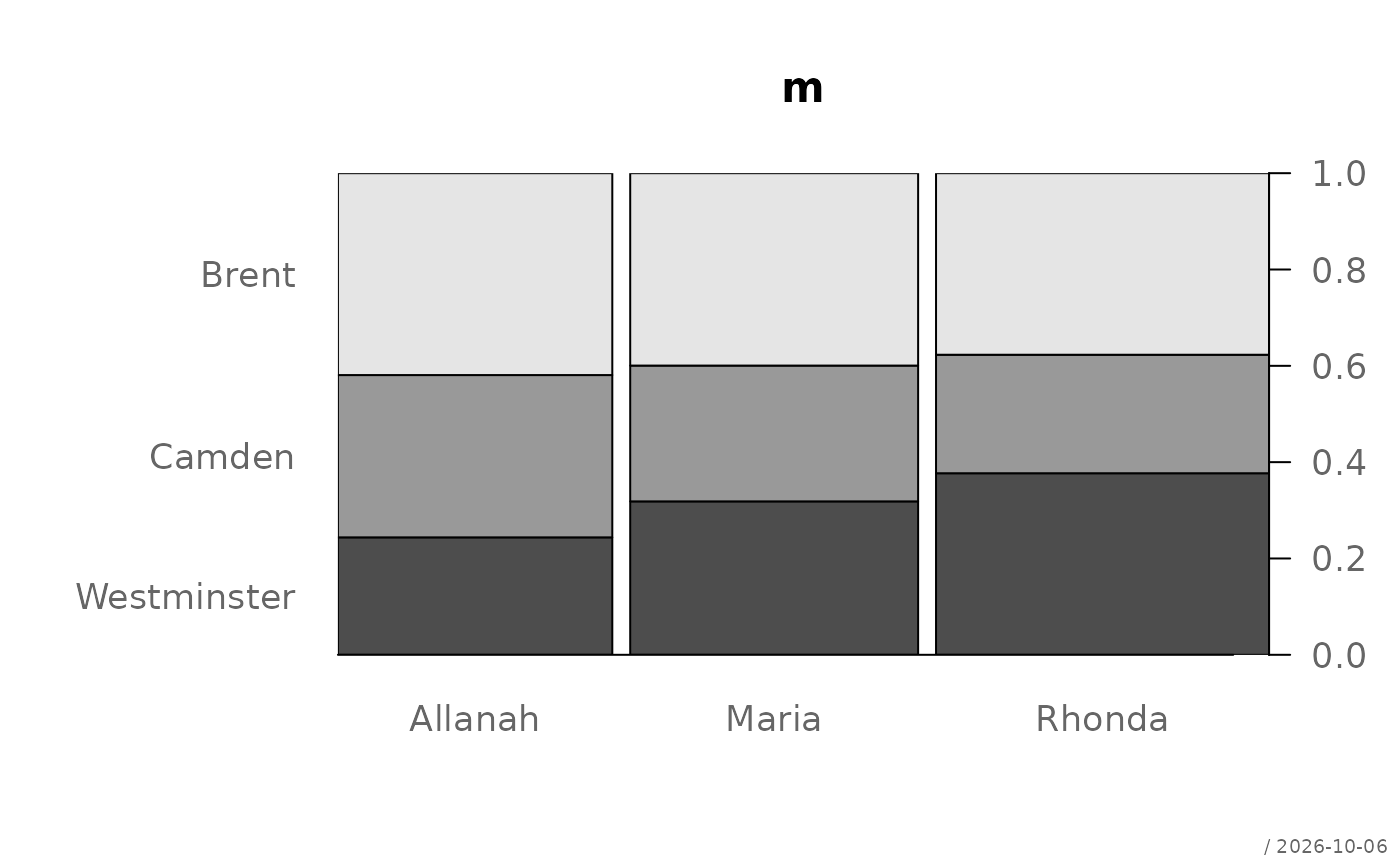
m <- matrix(c(153, 153, 167, 123, 108, 109, 89, 122, 167),
nrow = 3, byrow = TRUE,
dimnames = list(c("Brent","Camden","Westminster"),
c("Allanah","Maria","Rhonda")))
desc(m, verbose = 2)
#> ──────────────────────────────────────────────────────────────────────────────
#> m (matrix, array)
#>
#> Summary:
#> n: 1191, rows: 3, columns: 3
#>
#> Allanah Maria Rhonda Sum
#>
#> Brent freq 153 153 167 473
#> p.row 32.3% 32.3% 35.3% 39.7%
#>
#> Camden freq 123 108 109 340
#> p.row 36.2% 31.8% 32.1% 28.5%
#>
#> Westminster freq 89 122 167 378
#> p.row 23.5% 32.3% 44.2% 31.7%
#>
#> Sum freq 365 383 443 1191
#> p.row 30.6% 32.2% 37.2% 100.0%
#>
#>
#> Pearson's Chi-squared test:
#> X-squared = 17.905, df = 4, p-value = 0.001288
#> Log likelihood ratio (G-test) test of independence:
#> G = 18.099, df = 4, p-value = 0.001181
#> Mantel-Haenszel Chi-squared:
#> X-squared = 8.6654, df = 1, p-value = 0.003243
#>
#> Contingency Coeff. 0.122
#> Cramer V 0.087
#> Kendall Tau-b 0.073
#>
 # plots, see pharos::plot.Desc.table()
desc(tab, plotit = FALSE) |> plot(which = 4)
# plots, see pharos::plot.Desc.table()
desc(tab, plotit = FALSE) |> plot(which = 4)