Describe a Numeric-Numeric Relationship

Computes, prints and plots a comprehensive bivariate description for two quantitative variables. The function is dispatched automatically by desc(y ~ x, data) when both y and x are numeric.

Usage

.descNN(y, x, conf.level = 0.95)

# S3 method for class 'Desc.nn'
print(x, verbose = NULL, ...)

# S3 method for class 'Desc.nn'
plot(x, main = x$meta$main, which = 1, verbose = NULL, ...)

Arguments

x: numeric predictor for .descNN(), or an object of class "Desc.nn" for the print and plot methods
verbose: integer controlling the amount of printed output (1, 2, or 3). NULL (default) falls back to x$meta$verbose \%||\% getOption("DescTools.verbose", 2). Has no effect on plot().
...: further arguments. In plot() they are passed on to the plot function selected by which (see section Plots, where each function is linked). They go unchanged to every selected plot, so arguments specific to one function, such as type for pharos::plotDens2D(), belong with a single which.
main: main title for the plot. Defaults to the title stored in x$meta$main.
which: integer vector selecting the plots to draw, one plot per element, see section Plots. Default 1.
y: numeric response variable
conf.level: confidence level for interval estimates (default 0.95)

Value

.descNN() returns an object of class c("Desc.nn", "Desc"). Its lm$intercept and lm$slope components contain:

est: point estimate of the coefficient
lci: lower confidence interval bound
uci: upper confidence interval bound
p: p-value

The print and plot methods return x invisibly.

Details

Print output by verbose level:

verbose = 1: Summary (n, missings), Pearson r and Spearman r each with confidence interval and effect size label, linear regression coefficients (estimate, CI, significance) and R².
verbose = 2 (default): All of the above, plus residual standard error and Shapiro-Wilk test on residuals.
verbose = 3: All of the above, plus Breusch-Pagan test for heteroscedasticity and Cook's distance summary.

Confidence intervals are reported throughout instead of standard errors and t-values, using confint() for regression coefficients and corCI() (Fisher z-transform) for correlations.

Effect size labels for correlations follow Cohen (1988):

`negligible`	\|r\| < 0.10
`small`	0.10 $\le$ \|r\| < 0.30
`moderate`	0.30 $\le$ \|r\| < 0.50
`large`	\|r\| $\ge$ 0.50

Plots

plot() draws one of four displays of the joint distribution, selected by which. All arguments in ... go straight to the underlying function; its help page lists what can be set.

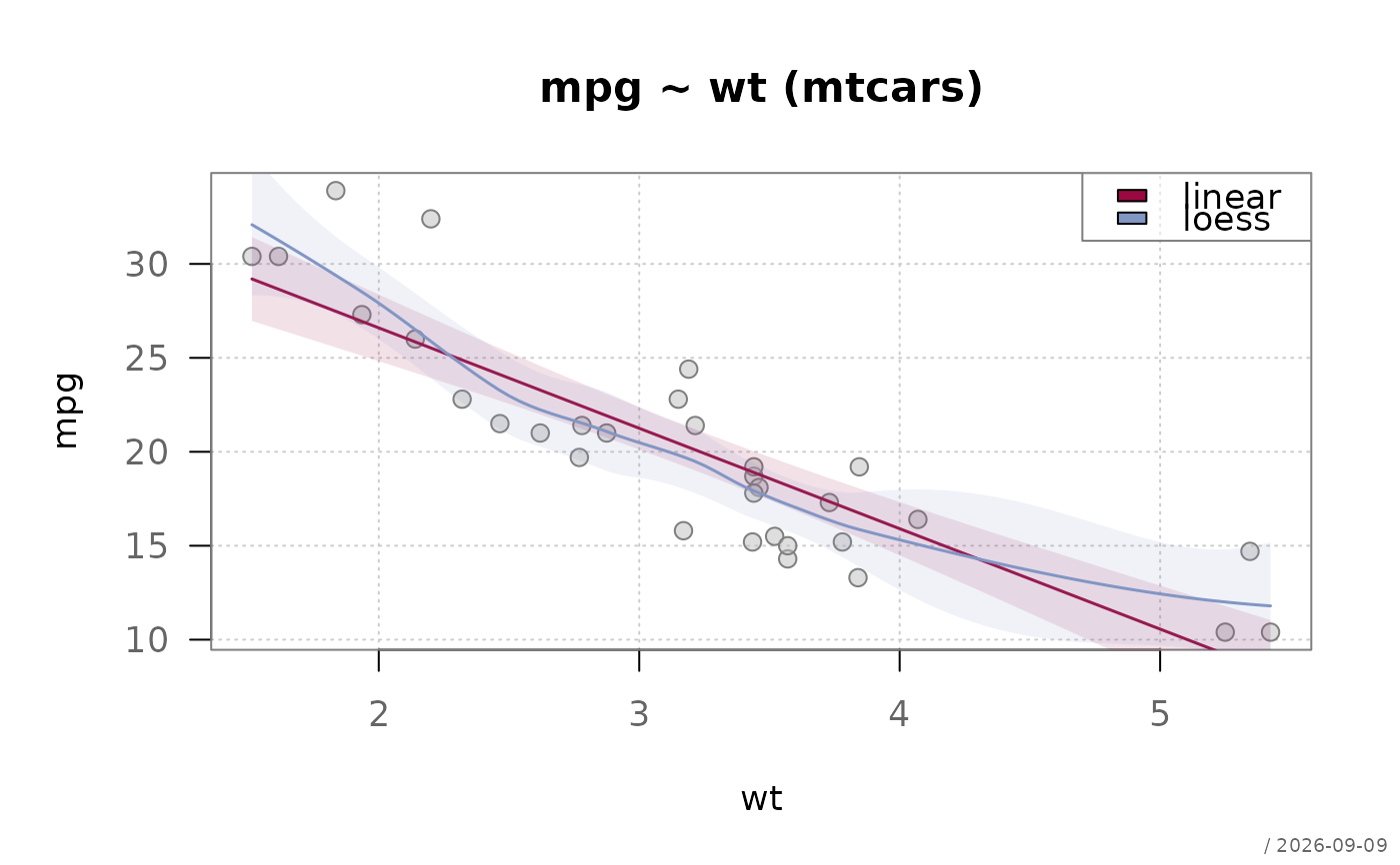
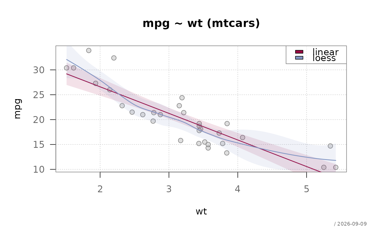
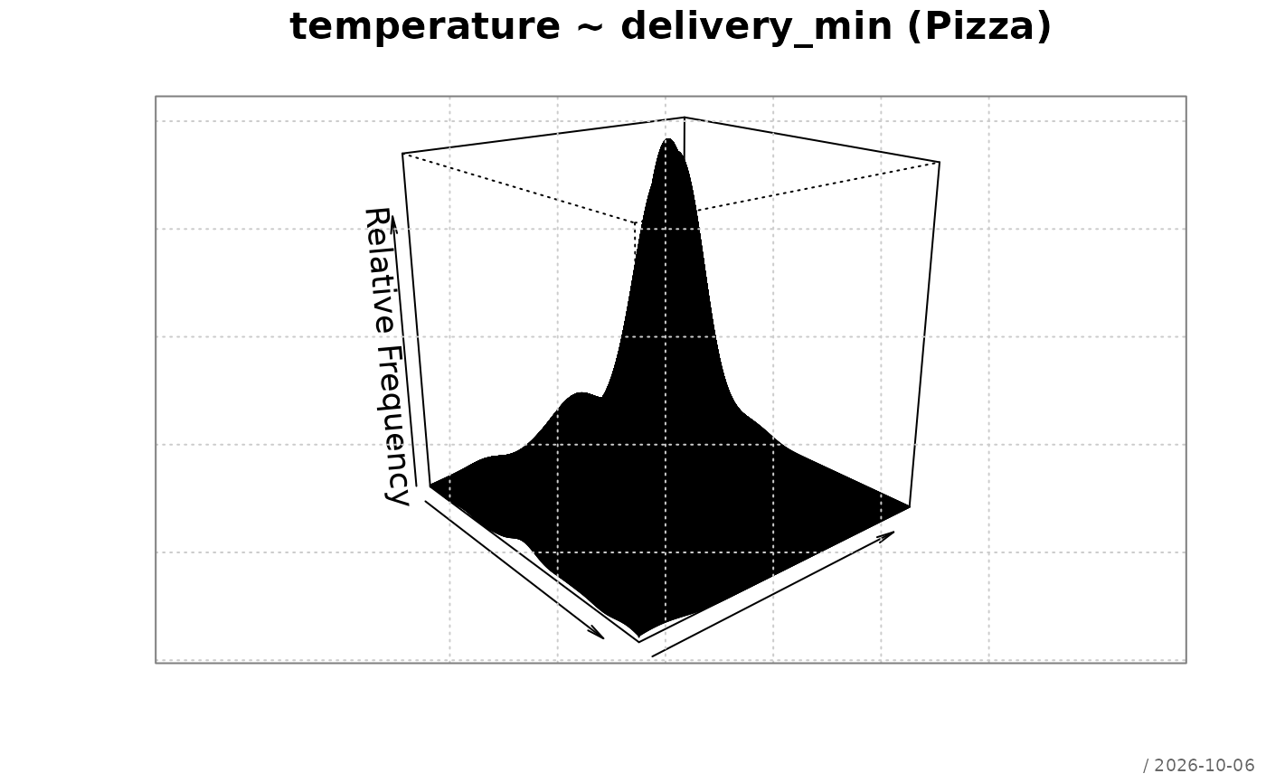
which = 1: Scatterplot of response against predictor, drawn by pharos::plotXY(). Axes are labelled with the variable names; point style, regression line and smoothers are controlled there.
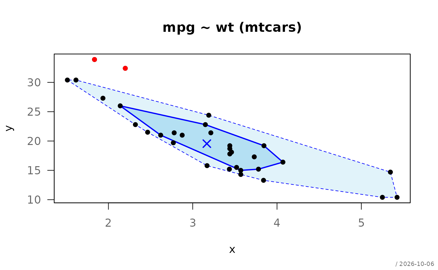
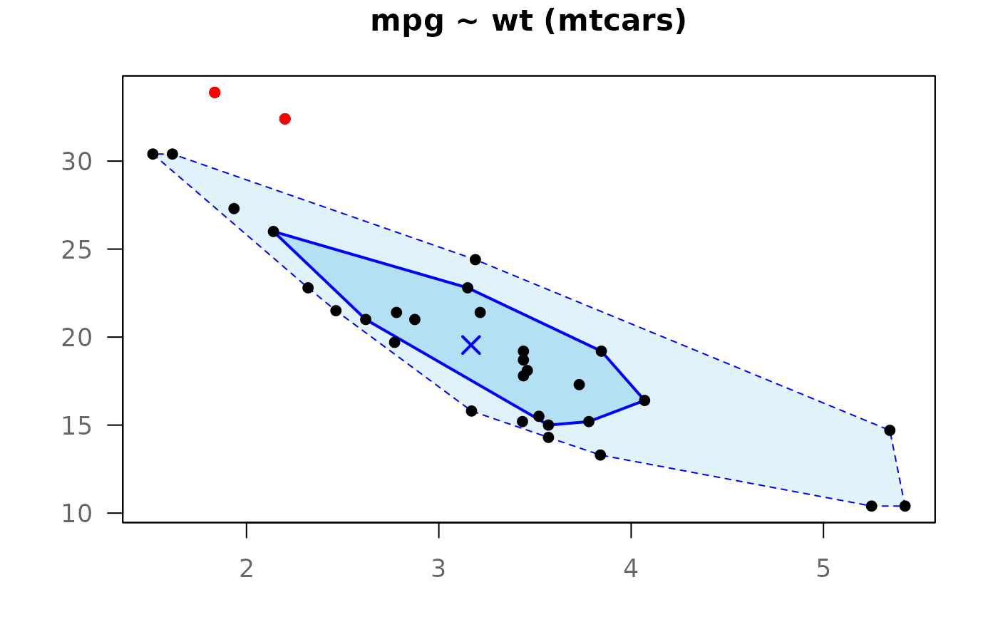
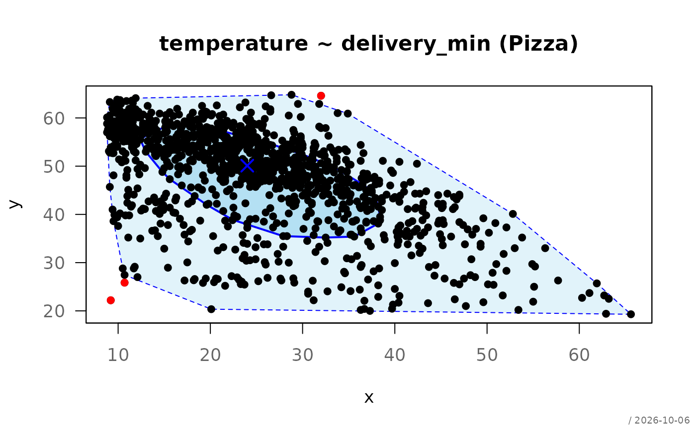
which = 2: Two-dimensional kernel density estimate on the complete cases, drawn by pharos::plotDens2D(). Its type argument switches the display, e.g. type = "contour", "image" or "persp".
which = 3: Bagplot (bivariate boxplot: bag with the inner half of the data, fence, outliers), drawn by pharos::plotBag().
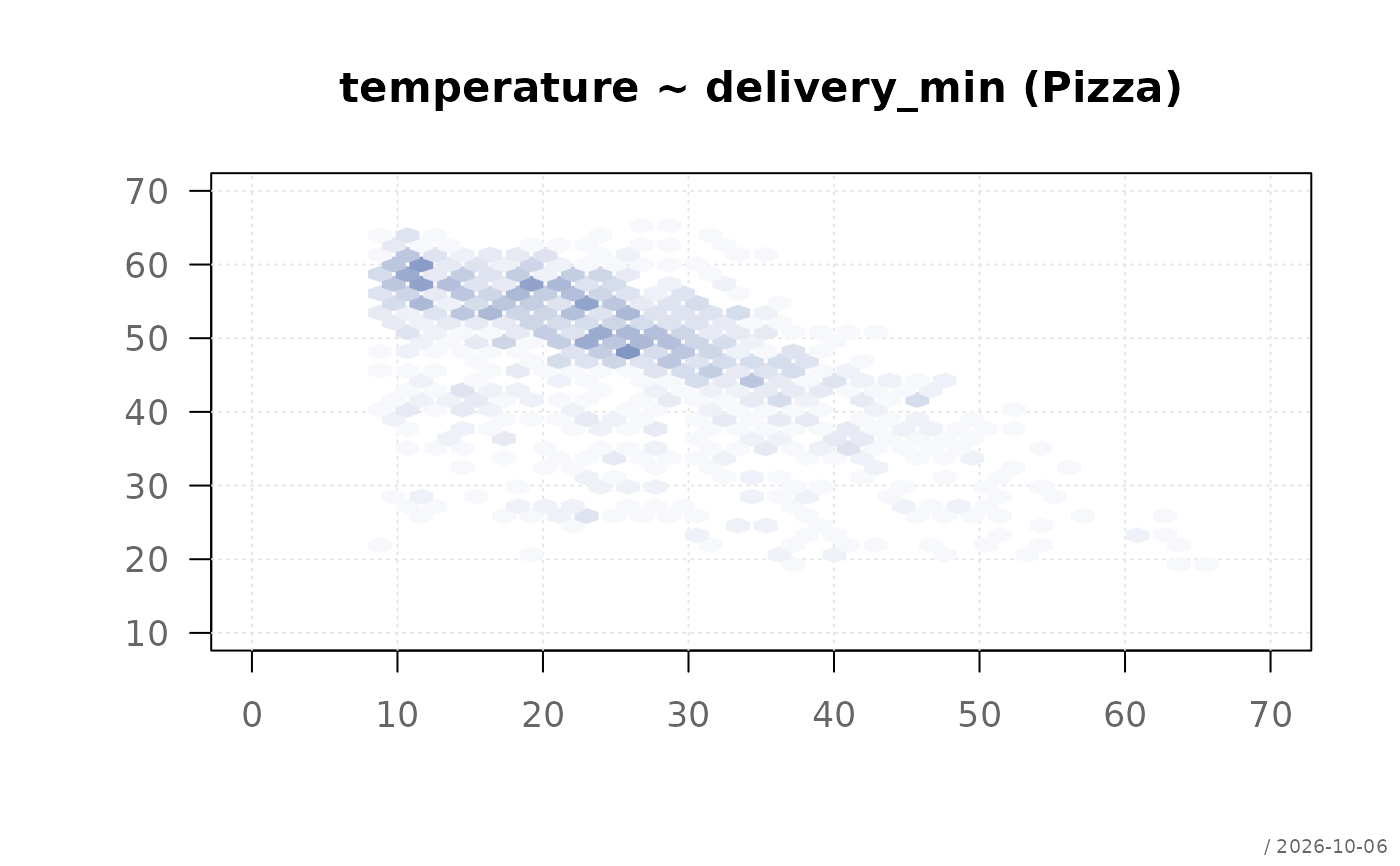
which = 4: Hexagonal binning, drawn by pharos::plotHexbin(); the choice for large n, where points in a scatterplot overplot.

main defaults to the title stored in the object and is passed to every plot.

References

Cohen, J. (1988). Statistical Power Analysis for the Behavioral Sciences (2nd ed.). Lawrence Erlbaum Associates.

Breusch, T.S. and Pagan, A.R. (1979). A simple test for heteroscedasticity and random coefficient variation. Econometrica, 47, 1287–1294.

Examples

# basic usage via desc()
desc(temperature ~ delivery_min, Pizza)
#> ────────────────────────────────────────────────────────────────────────────── 
#> temperature ~ delivery_min (Pizza) (Desc.nn)
#> 
#> Summary:
#> pairs: 1209, valid: 1170 (96.8%), missings: 39 (3.2%)
#> 
#> Pearson  r:  -0.575  (-0.612, -0.536)  ***  large
#> Spearman r:  -0.573  (-0.611, -0.534)  ***  large
#> 
#> Linear regression:
#>   Intercept:   61.4190  ( 60.2237,  62.6142)  ***
#>   Slope:       -0.5347  ( -0.5783,  -0.4910)  ***
#>   R²: 0.331   adj. R²: 0.330   p: <0.001
#>   Residual SE: 8.1324 on 1168 df
#>   Shapiro-Wilk on residuals: W = 0.910,  p = <0.001
#> 


# more detail
desc(temperature ~ delivery_min, Pizza, verbose = 3)
#> ────────────────────────────────────────────────────────────────────────────── 
#> temperature ~ delivery_min (Pizza) (Desc.nn)
#> 
#> Summary:
#> pairs: 1209, valid: 1170 (96.8%), missings: 39 (3.2%)
#> 
#> Pearson  r:  -0.575  (-0.612, -0.536)  ***  large
#> Spearman r:  -0.573  (-0.611, -0.534)  ***  large
#> 
#> Linear regression:
#>   Intercept:   61.4190  ( 60.2237,  62.6142)  ***
#>   Slope:       -0.5347  ( -0.5783,  -0.4910)  ***
#>   R²: 0.331   adj. R²: 0.330   p: <0.001
#>   Residual SE: 8.1324 on 1168 df
#>   Shapiro-Wilk on residuals: W = 0.910,  p = <0.001
#> 
#>   Breusch-Pagan test: BP = 2.2987,  df = 1,  p = 0.129
#>   Cook's distance: max = 0.0248,  n > 4/n threshold: 71
#> 


# store result, print and plot separately
d <- desc(temperature ~ delivery_min, Pizza, plotit = FALSE)
print(d, verbose = 1)
#> ────────────────────────────────────────────────────────────────────────────── 
#> temperature ~ delivery_min (Pizza) (Desc.nn)
#> 
#> Summary:
#> pairs: 1209, valid: 1170 (96.8%), missings: 39 (3.2%)
#> 
#> Pearson  r:  -0.575  (-0.612, -0.536)  ***  large
#> Spearman r:  -0.573  (-0.611, -0.534)  ***  large
#> 
#> Linear regression:
#>   Intercept:   61.4190  ( 60.2237,  62.6142)  ***
#>   Slope:       -0.5347  ( -0.5783,  -0.4910)  ***
#>   R²: 0.331   adj. R²: 0.330   p: <0.001
#> 

# the four plots
plot(d, which = 1)                     # scatterplot       -> plotXY()
plot(d, which = 2)                     # 2D density        -> plotDens2D()

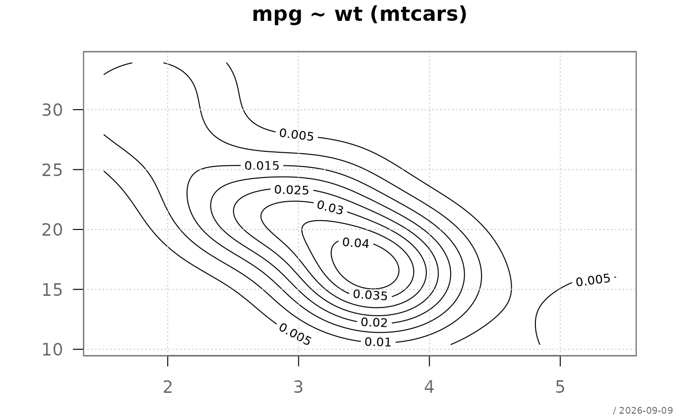plot(d, which = 2, type = "contour")
plot(d, which = 2, type = "image")

plot(d, which = 2, type = "persp")

plot(d, which = 3)                     # bagplot           -> plotBag()

plot(d, which = 4)                     # hexagonal binning -> plotHexbin()


# pipe
desc(mpg ~ wt, mtcars) |> plot(which = 3)