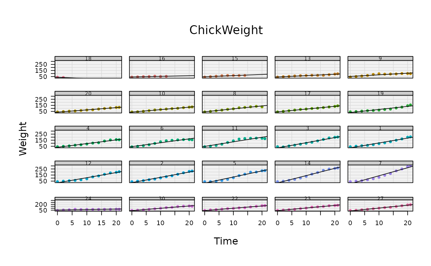
Facet Panel Matrix in Base Graphics

Draws a lattice-like matrix of panels in base graphics with identical plot region sizes, panel strips, axes on the outer panels only and a user-supplied panel function for the content. Panel gaps are defined in margin lines and remain exact, independent of device size and strip height, as the strip space is reserved separately in the layout.

Usage

plotFacet(
  samples,
  dim,
  panelFun,
  cols = NULL,
  stripLabels = NULL,
  main = "",
  xlab = "",
  ylab = "",
  xlim = NULL,
  ylim = NULL,
  mar = c(2.5, 2.5, 0.5, 0.5),
  oma = c(3, 3, 4, 1.2),
  horiz = 1,
  vert = NULL,
  strip = TRUE,
  bg = "grey95",
  grid = TRUE,
  cex = 0.66,
  pch = 16,
  ...
)

Arguments

samples: a list of samples, each a list (or data.frame) with components x and y.
dim: integer vector of length 2, the number of rows and columns of the panel matrix, c(nrow, ncol).
panelFun: the panel function, called per panel as panelFun(x, y, col, pch, ...) with a fully set up coordinate system. Components of a sample beyond x and y are passed on under their own names, so a panel can carry per-panel data of its own - confidence bounds, weights, labels. They are only passed to a panelFun that can accept them (a matching formal, or ...), so panel functions written for the two-component form keep working unchanged.
cols: the colors for the panels, recycled to the number of samples. Default is hcl.colors(n, "Dark 3").
stripLabels: the labels for the panel strips. Default is names(samples) where the samples are named, otherwise the sequence along samples.
main: the main title, placed in the outer margin.
xlab, ylab: the axis labels, placed in the outer margins.
xlim, ylim: the axis limits. A numeric vector of length 2 (or NULL, the default, for the range over all samples) binds every panel to the same scale. "free" gives each panel its own scale, taken from its own sample. A list of length 2 vectors, one per sample, does the same with limits you choose; a list of length 1 is recycled. See the section on free scales.
mar: the margins around the whole panel matrix in lines, c(bottom, left, top, right). The bottom and left margins hold the axis annotation of the outer panels.
oma: the outer margins in lines, holding xlab, ylab and main.
horiz: the horizontal gap between adjacent columns in margin lines.
vert: the vertical gap between adjacent rows in margin lines. Default is horiz, yielding physically equal gaps.
strip: controls the panel strips, evaluated by bedrock::callIf: TRUE (default) draws strips with default settings, FALSE/NULL/NA suppresses them (no space is reserved), a named list is passed as arguments to titleRect(), e.g. list(bg = "steelblue", col = "white", line = 1.5). The label argument is set per panel from stripLabels and cannot be overridden.
bg: the background color of the plot regions.
grid: controls the grid lines, evaluated by bedrock::callIf: TRUE (default) draws grid lines at the positions of axTicks() with default settings (col = "grey85", lwd = 0.8), FALSE/NULL/NA suppresses them, a named list is passed as arguments to abline(), e.g. list(col = "white", lty = "dotted"). The default positions v and h can be overridden, e.g. list(v = seq(0, 20, 5)).
cex: the character expansion used inside the panels (axis annotation, strip labels, panel content) and as unit for the panel margin lines. Default is 0.66, matching R's own reduction in multi-figure layouts. Set deterministically after each plot.new(), see Details.
pch: the plotting character, passed to panelFun.
...: the dots are passed to panelFun.

Value

Invisibly returns a list with the realized geometry: horiz, vert, strip_line (reserved strip height in lines) and the common plot region size plot_width_in, plot_height_in in inches.

Details

The available device area inside the outer margins is partitioned with layout() such that all plot regions have exactly the same size in inches. The horizontal gap between two adjacent columns is horiz margin lines, the vertical gap between two adjacent rows is vert lines. Since margin lines have the same physical size in both directions, horiz == vert yields visually equal gaps.

Bound and free scales

By default all panels share one coordinate system, and the axes are drawn on the outer panels only - the arrangement that makes small multiples comparable at a glance.

Passing xlim = "free" - or a list of limits, for control over the individual panels - frees that dimension: every panel gets its own limits, and with them its own axis, because an outer axis would no longer describe the panels above or beside it. The layout answers for this - a freed dimension reserves the full mar on every panel edge that now carries annotation, not just on the outer ones, so the panels stay equal in size and the tick labels have room.

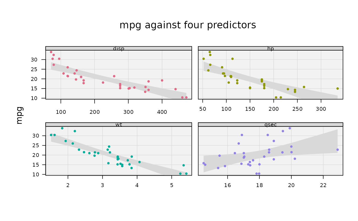
Free scales cost what they free: panels can no longer be compared by position, only by shape. The natural case is a set of diagnostics of one model against different predictors - the residual scale is shared and worth comparing, the predictor scales are not commensurable at all.

The strip is drawn with titleRect() above each panel. Its height (line argument of titleRect) is reserved in the top margin of every panel, so the strip never eats into the gap between the rows.

Note that plot.new() silently reduces cex (and with it csi, the physical size of a margin line) in layouts with more than two regions, which would make the realized panel margins deviate from the computed layout. The function therefore controls the character size deterministically via its cex argument and sets the panel margins in inches (mai/omi), so that all plot regions are exactly equal in size.

Examples

samples <- lapply(split(ChickWeight, ChickWeight$Chick)[1:25],
                  function(z) list(x = z$Time, y = z$weight))

my_panel <- function(x, y, col, pch = 16, ...) {
  points(x, y, pch = pch, col = col)
  abline(lm(y ~ x), lwd = 1)
}

plotFacet(samples, dim = c(5, 5), panelFun = my_panel,
           xlab = "Time", ylab = "Weight", main = "ChickWeight",
           strip = list(bg = "grey80", cex = 0.8))


# free x scales: mpg against four predictors, each on its own range,
# with a shared y scale. The regression band travels in the samples and
# reaches the panel function under its own names.
vars <- c("disp", "hp", "wt", "qsec")

samples <- lapply(vars, function(v) {
  ord <- order(mtcars[[v]])
  ci  <- predict(lm(reformulate(v, "mpg"), mtcars), interval = "confidence")
  list(x = mtcars[[v]][ord], y = mtcars$mpg[ord],
       lci = ci[ord, "lwr"], uci = ci[ord, "upr"])
})

panelBand <- function(x, y, lci, uci, col, pch = 16, ...) {
  polygon(c(x, rev(x)), c(uci, rev(lci)), col = "grey85", border = NA)
  points(x, y, col = col, pch = pch)
}

plotFacet(setNames(samples, vars), dim = c(2, 2), panelFun = panelBand,
          xlim = "free", ylab = "mpg",
          main = "mpg against four predictors")