Add a linear regression line to an existing plot. The function first
calculates predictions from an lm object and then adds the fitted
line together with optional confidence and prediction bands.
Usage
# S3 method for class 'lm'
lines(
  x,
  col = pal()[1],
  lwd = 2,
  lty = "solid",
  type = "l",
  n = 100,
  cband = list(conf.level = 0.95),
  pband = NA,
  xpred = NULL,
  ...
)

# S3 method for class 'lmlog'
lines(
  x,
  col = pal()[1],
  lwd = 2,
  lty = "solid",
  type = "l",
  n = 100,
  cband = list(conf.level = 0.95),
  pband = NA,
  xpred = NULL,
  ...
)
Arguments
- x
linear model object as returned by
lm().- col
line color. Defaults to
pal()[1].- lwd
line width.
- lty
line type.
- type
plotting type passed to
lines().- n
number of points used for plotting the fit.
- cband
controls the confidence band. May be
TRUE,FALSE,NULL,NA, or a named list. The confidence level is specified viaconf.level, all other elements are graphical parameters of the band. Default islist(conf.level=0.95).- pband
controls the prediction band, as
cband. Default isNA.- xpred
optional numeric vector defining the range over which predictions should be calculated.
- ...
further graphical parameters passed to
lines()for the fitted line.
Details
In contrast to abline(), polynomial models and transformed
predictors are supported as long as the model contains exactly one predictor
variable. A polynomial, y ~ poly(x, 2) or y ~ x + I(x^2), is drawn
against x; a single transformed term such as y ~ log(x) is drawn
against the transformed values, matching plot(y ~ log(x)).
Confidence and prediction bands are controlled via cband and
pband. These arguments can be:
FALSE,NULLorNA: suppress the bandTRUE: draw the band with default settingsa named list: customize the band appearance and confidence level
See also
Other graphics.trendlines:
lines.loess(),
splineCI
Examples
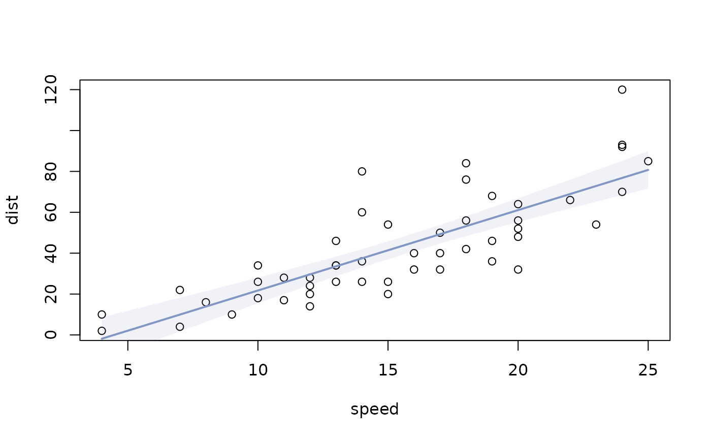
plot(dist ~ speed, cars)
lines(lm(dist ~ speed, cars))
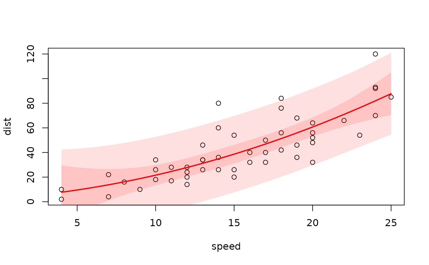
 # polynomial model with a 99% confidence band and a prediction band
plot(dist ~ speed, cars)
lines(lm(dist ~ poly(speed, 2), cars), col = "red",
cband = list(conf.level = 0.99), pband = TRUE)
# polynomial model with a 99% confidence band and a prediction band
plot(dist ~ speed, cars)
lines(lm(dist ~ poly(speed, 2), cars), col = "red",
cband = list(conf.level = 0.99), pband = TRUE)
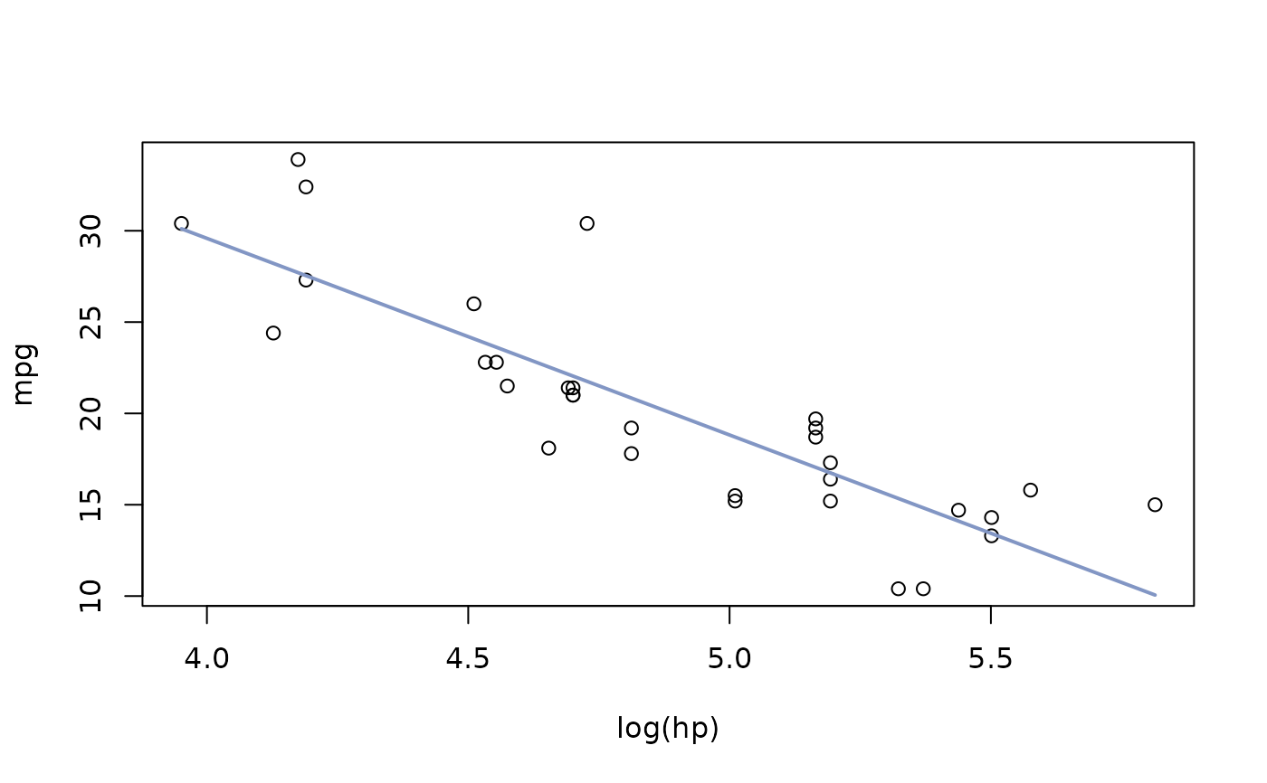
 # transformed predictor, no bands
plot(mpg ~ log(hp), mtcars)
lines(lm(mpg ~ log(hp), mtcars), cband = FALSE)
# transformed predictor, no bands
plot(mpg ~ log(hp), mtcars)
lines(lm(mpg ~ log(hp), mtcars), cband = FALSE)