Comparison Table For Linear Models
TMod.RdCollect the coefficients and some qualifying statistics of linear models and organize it in a table for comparison and reporting. The function supports linear and general linear models.
TMod(..., FUN = NULL, order = NA, verb = FALSE)

ModSummary(x, ...)

# S3 method for class 'lm'
ModSummary(x, conf.level = 0.95, ...)
# S3 method for class 'glm'
ModSummary(x, conf.level = 0.95, use.profile = TRUE, ...)

# S3 method for class 'TMod'
plot(x, terms = NULL, intercept = FALSE, ...)
# S3 method for class 'TMod'
print(x, digits = 3, na.form = "-", verb = NULL, ...)
Arguments
- x
a (general) linear model object.
- ...
a list of (general) linear models.
- conf.level
the level for the confidence intervals.
- FUN
function with arguments
est,se,tval,pval,lci,ucito display the coefficients. The default function will display the coefficient and significance stars for the p-values.- order
row of the results table to be used as order for the models (as typically "AIC"). Can be any label in the first column of the results table. Default is
NAfor no special order.- verb
logical, determining whether the full set of model performance indicators (
TRUE) or a reduced set should be displayed (FALSEis default).- terms
a vector with the terms of the model formula to be plotted. By default this will be all of them.
- use.profile
logical. Defines if profile approach should be used, which normally is a good choice for small datasets. Calculating profile can however take ages for large datasets and not be necessary there. So we can fallback to normal confidence intervals.
- intercept
logical, defining whether the intercept should be plotted (default is
FALSE).- digits
integer, the desired (fixed) number of digits after the decimal point. Unlike
formatCyou will always get this number of digits even if the last digit is 0.- na.form
character, string specifying how
NAs should be specially formatted. If set toNULL(default) no special action will be taken.
Details
In order to compare the coefficients of linear models, the user is left to his own devices. R offers no support in this respect. TMod() jumps into the breach and displays the coefficients of several models in tabular form. For this purpose, different quality indicators for the models are displayed, so that a comprehensive comparison of the models is possible. In particular, it is easy to see the effect that adding or omitting variables has on forecast quality.
A plot function for a TMod object will produce a dotchart with the coefficients and their confidence intervals.
Value
character table
See also
Examples
r.full <- lm(Fertility ~ . , swiss)
r.nox <- lm(Fertility ~ . -Examination - Catholic, swiss)
r.grp <- lm(Fertility ~ . -Education - Catholic + CutQ(Catholic), swiss)
r.gam <- glm(Fertility ~ . , swiss, family=Gamma(link="identity"))
r.gama <- glm(Fertility ~ .- Agriculture , swiss, family=Gamma(link="identity"))
r.gaml <- glm(Fertility ~ . , swiss, family=Gamma(link="log"))
TMod(r.full, r.nox, r.grp, r.gam, r.gama, r.gaml)
#> Waiting for profiling to be done...
#> Waiting for profiling to be done...
#> Waiting for profiling to be done...
#> coef r.full r.nox r.grp r.gam r.gama
#> 1 (Intercept) 66.915 *** 51.101 *** 53.411 *** 63.709 *** 48.790 ***
#> 2 Agriculture -0.172 * -0.026 -0.096 -0.175 * -
#> 3 Examination -0.258 - -0.872 *** -0.129 0.050
#> 4 Education -0.871 *** -0.857 *** - -0.944 *** -0.808 ***
#> 5 Catholic 0.104 ** - - 0.106 ** 0.089 *
#> 6 Infant.Mortality 1.077 ** 1.493 ** 1.796 *** 1.174 ** 1.290 **
#> 7 CutQ(Catholic)Q2 - - -0.035 - -
#> 8 CutQ(Catholic)Q3 - - -5.780 - -
#> 9 CutQ(Catholic)Q4 - - 5.939 - -
#> 10 ---
#> 11 adj.r.squared 0.671 0.536 0.552 - -
#> 12 AIC 326.072 340.485 341.398 327.012 331.347
#> 13 N 47 47 47 47 47
#> 14 NAs 0 0 0 0 0
#> 15 n vars 5 3 4 5 4
#> 16 n coef 6 4 7 6 5
#> 17 MAE 5.321 6.826 6.079 5.330 5.869
#> 18 RMSE 6.692 8.141 7.712 6.734 7.212
#> 19 McFadden - - - 0.163 0.146
#> r.gaml
#> 1 4.184 ***
#> 2 -0.002 *
#> 3 -0.003
#> 4 -0.015 ***
#> 5 0.001 *
#> 6 0.017 **
#> 7 -
#> 8 -
#> 9 -
#> 10
#> 11 -
#> 12 328.449
#> 13 47
#> 14 0
#> 15 5
#> 16 6
#> 17 5.458
#> 18 6.882
#> 19 0.159
# display confidence intervals
TMod(r.full, r.nox, r.gam, FUN = function(est, se, tval, pval, lci, uci){
gettextf("%s [%s, %s]",
Format(est, fmt=Fmt("num")),
Format(lci, digits=3),
Format(uci, digits=2)
)
})
#> Waiting for profiling to be done...
#> coef r.full r.nox
#> 1 (Intercept) 66.915 [45.294, 88.54] 51.101 [28.928, 73.27]
#> 2 Agriculture -0.172 [-0.314, -0.03] -0.026 [-0.173, 0.12]
#> 3 Examination -0.258 [-0.771, 0.25] -
#> 4 Education -0.871 [-1.241, -0.50] -0.857 [-1.205, -0.51]
#> 5 Catholic 0.104 [0.033, 0.18] -
#> 6 Infant.Mortality 1.077 [0.306, 1.85] 1.493 [0.608, 2.38]
#> 7 ---
#> 8 adj.r.squared 0.671 0.536
#> 9 AIC 326.072 340.485
#> 10 N 47 47
#> 11 NAs 0 0
#> 12 n vars 5 3
#> 13 n coef 6 4
#> 14 MAE 5.321 6.826
#> 15 RMSE 6.692 8.141
#> 16 McFadden - -
#> r.gam
#> 1 63.709 [44.294, 83.44]
#> 2 -0.175 [-0.318, -0.04]
#> 3 -0.129 [-0.626, 0.36]
#> 4 -0.944 [-1.252, -0.63]
#> 5 0.106 [0.035, 0.18]
#> 6 1.174 [0.479, 1.84]
#> 7
#> 8 -
#> 9 327.012
#> 10 47
#> 11 0
#> 12 5
#> 13 6
#> 14 5.330
#> 15 6.734
#> 16 0.163
# cbind interface is not supported!!
# d.titanic <- reshape(as.data.frame(Titanic),
# idvar = c("Class","Sex","Age"),
# timevar="Survived",
# direction = "wide")
#
# r.glm0 <- glm(cbind(Freq.Yes, Freq.No) ~ 1, data=d.titanic, family="binomial")
# r.glm1 <- glm(cbind(Freq.Yes, Freq.No) ~ Class, data=d.titanic, family="binomial")
# r.glm2 <- glm(cbind(Freq.Yes, Freq.No) ~ ., data=d.titanic, family="binomial")
d.titanic <- Untable(Titanic)
r.glm0 <- glm(Survived ~ 1, data=d.titanic, family="binomial")
r.glm1 <- glm(Survived ~ Class, data=d.titanic, family="binomial")
r.glm2 <- glm(Survived ~ ., data=d.titanic, family="binomial")
TMod(r.glm0, r.glm1, r.glm2)
#> Waiting for profiling to be done...
#> Waiting for profiling to be done...
#> Waiting for profiling to be done...
#> coef r.glm0 r.glm1 r.glm2
#> 1 (Intercept) -0.740 *** 0.509 *** 0.685 *
#> 2 Class2nd - -0.856 *** -1.018 ***
#> 3 Class3rd - -1.596 *** -1.778 ***
#> 4 ClassCrew - -1.664 *** -0.858 ***
#> 5 SexFemale - - 2.420 ***
#> 6 AgeAdult - - -1.062 ***
#> 7 ---
#> 8 AIC 2771.457 2596.555 2222.061
#> 9 N 2201 2201 2201
#> 10 NAs 0 0 0
#> 11 n vars 0 1 3
#> 12 McFadden 0.000 0.065 0.202
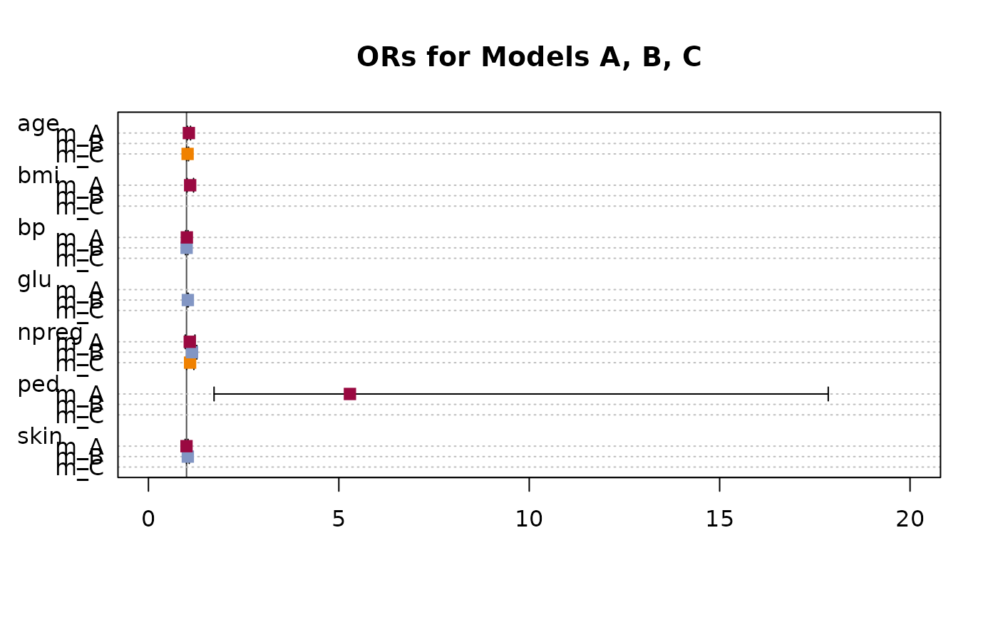
# plot OddsRatios
d.pima <- MASS::Pima.tr2
r.a <- glm(type ~ npreg + bp + skin + bmi + ped + age, data=d.pima, family=binomial)
r.b <- glm(type ~ npreg + glu + bp + skin, data=d.pima, family=binomial)
r.c <- glm(type ~ npreg + age, data=d.pima, family=binomial)
or.a <- OddsRatio(r.a)
or.b <- OddsRatio(r.b)
or.c <- OddsRatio(r.c)
# create the model table
tm <- TMod(m_A=or.a, m_B=or.b, m_C=or.c)
# .. and plotit
plot(tm, main="ORs for Models A, B, C", intercept=FALSE,
pch=15, col=c(DescTools::hred, DescTools::hblue, DescTools::horange),
panel.first=abline(v=1, col="grey30"))