Odds Ratio Estimation and Confidence Intervals
OddsRatio.RdCalculates odds ratio by unconditional maximum likelihood estimation (wald),
conditional maximum likelihood estimation (mle) or median-unbiased estimation (midp).
Confidence intervals are calculated using normal approximation (wald) and exact methods
(midp, mle).
OddsRatio(x, conf.level = NULL, ...)

# S3 method for class 'glm'
OddsRatio(x, conf.level = NULL, digits = 3, use.profile = FALSE, ...)

# S3 method for class 'multinom'
OddsRatio(x, conf.level = NULL, digits = 3, ...)

# S3 method for class 'zeroinfl'
OddsRatio(x, conf.level = NULL, digits = 3, ...)

# Default S3 method
OddsRatio(x, conf.level = NULL, y = NULL, method = c("wald", "mle", "midp"),
          interval = c(0, 1000), ...)
Arguments
- x
a vector or a \(2 \times 2\) numeric matrix, resp. table.
- y
NULL (default) or a vector with compatible dimensions to
x. If y is provided,table(x, y, ...)will be calculated.- digits
the number of fixed digits to be used for printing the odds ratios.
- method
method for calculating odds ratio and confidence intervals. Can be one out of "
wald", "mle", "midp". Default is"wald"(not because it is the best, but because it is the most commonly used.)- conf.level
confidence level. Default is
NAfor tables and numeric vectors, meaning no confidence intervals will be reported. 0.95 is used as default for models.- interval
interval for the function
unirootthat finds the odds ratio median-unbiased estimate andmidpexact confidence interval.- use.profile
logical. Defines if profile approach should be used, which normally is a good choice. Calculating profile can however take ages for large datasets and not be necessary there. So we can fallback to normal confidence intervals.
- ...
further arguments are passed to the function
table, allowing i.e. to setuseNA. This refers only to the vector interface.
Details
If a \(2 \times 2\) table is provided the following table structure is preferred:
                    disease=1   disease=0
    exposed=1          n11         n10
    exposed=0          n01         n00
however, for odds ratios the following table is equivalent:
                    disease=0   disease=1
    exposed=0 (ref)    n00         n01
    exposed=1          n10         n11
If the table to be provided to this function is not in the
preferred form, the function Rev() can be used to "reverse" the table rows, resp.
-columns. Reversing columns or rows (but not both) will lead to the inverse of the odds ratio.
In case of zero entries, 0.5 will be added to the table.
Value
a single numeric value if conf.level is set to NA
a numeric vector with 3 elements for estimate, lower and upper confidence interval if conf.level is provided
References
Kenneth J. Rothman and Sander Greenland (1998): Modern Epidemiology, Lippincott-Raven Publishers
Kenneth J. Rothman (2002): Epidemiology: An Introduction, Oxford University Press
Nicolas P. Jewell (2004): Statistics for Epidemiology, 1st Edition, 2004, Chapman & Hall, pp. 73-81
Agresti, Alan (2013) Categorical Data Analysis. NY: John Wiley and Sons, Chapt. 3.1.1
See also
Examples
# Case-control study assessing whether exposure to tap water
# is associated with cryptosporidiosis among AIDS patients
tab <- matrix(c(2, 29, 35, 64, 12, 6), 3, 2, byrow=TRUE)
dimnames(tab) <- list("Tap water exposure" = c("Lowest", "Intermediate", "Highest"),
"Outcome" = c("Case", "Control"))
tab <- Rev(tab, margin=2)
OddsRatio(tab[1:2,])
#> [1] 7.929688
OddsRatio(tab[c(1,3),])
#> [1] 29
OddsRatio(tab[1:2,], method="mle")
#> [1] 7.836979
OddsRatio(tab[1:2,], method="midp")
#> [1] 7.355436
OddsRatio(tab[1:2,], method="wald", conf.level=0.95)
#> odds ratio lwr.ci upr.ci
#> 7.929688 1.785414 35.218699
# in case of zeros consider using glm for calculating OR
dp <- data.frame (a=c(20, 7, 0, 0), b=c(0, 0, 0, 12), t=c(1, 0, 1, 0))
fit <- glm(cbind(a, b) ~ t, data=dp, family=binomial)
exp(coef(fit))
#> (Intercept) t
#> 0.5833333 648881106.9538907
# calculation of log oddsratios in a 2x2xk table
migraine <- xtabs(freq ~ .,
cbind(expand.grid(treatment=c("active","placebo"),
response=c("better","same"),
gender=c("female","male")),
freq=c(16,5,11,20,12,7,16,19))
)
log(apply(migraine, 3, OddsRatio))
#> female male
#> 1.7609878 0.7108468
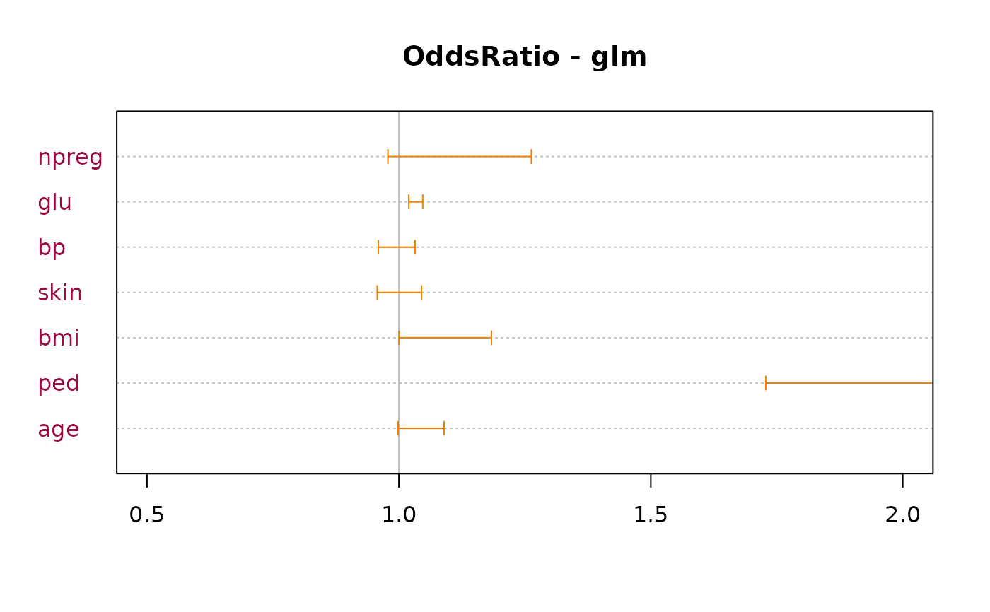
# OddsRatio table for logistic regression models
r.glm <- glm(type ~ ., data=MASS::Pima.tr2, family=binomial)
OddsRatio(r.glm)
#>
#> Call:
#> glm(formula = type ~ ., family = binomial, data = MASS::Pima.tr2)
#>
#> Odds Ratios:
#> or or.lci or.uci Pr(>|z|)
#> (Intercept) 0.000 0.000 0.002 3.38e-08 ***
#> npreg 1.109 0.977 1.259 0.1107
#> glu 1.033 1.019 1.046 2.22e-06 ***
#> bp 0.995 0.960 1.032 0.7971
#> skin 0.998 0.955 1.043 0.9321
#> bmi 1.087 1.000 1.182 0.0509 .
#> ped 6.174 1.675 22.755 0.0062 **
#> age 1.042 0.998 1.088 0.0623 .
#> ---
#> Signif. codes: 0 '***' 0.001 '**' 0.01 '*' 0.05 '.' 0.1 ' ' 1
#>
#> Brier Score: 0.147 Nagelkerke R2: 0.447
#>
plot(OddsRatio(r.glm), xlim=c(0.5, 2), main="OddsRatio - glm", pch=NA,
lblcolor=DescTools::hred, args.errbars=list(col=DescTools::horange, pch=21,
col.pch=DescTools::hblue,
bg.pch=DescTools::hyellow, cex.pch=1.5))