Plot Probability Distribution

Produce a plot from a probability distribution with shaded areas. This is often needed in theory texts for classes in statistics.

PlotProbDist(breaks, FUN, 
             blab = NULL, main = "", xlim = NULL, col = NULL, density = 7, 
             alab = LETTERS[1:(length(breaks) - 1)], 
             alab_x = NULL, alab_y = NULL, ylab = "density", ...)

Arguments

breaks

a numeric vector containing the breaks of different areas. The start and end must not be infinity.

FUN

the (typically) distribution function

blab

text for labelling the breaks

main

main title for the plot

xlim

the x-limits for the plot

col

the color for the shaded areas

density

the density for the shaded areas

alab

the labels for areas

alab_x

the x-coord for the area labels

alab_y

the y-coord for the area labels, if left to default they will be placed in the middle of the plot

ylab

the label for they y-axis

...

further parameters passed to internally used function curve()

Details

The function sets up a two-step plot procedure based on curve() and Shade() with additional labelling for convenience.

Value

nothing returned

Author

Andri Signorell <andri@signorell.net>

See also

Shade, curve, polygon

Examples

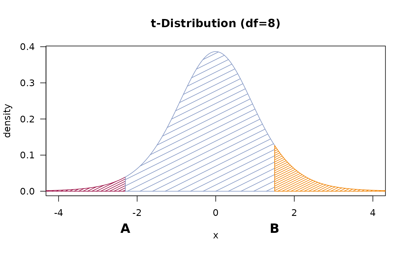
# plot t-distribution
PlotProbDist(breaks=c(-6, -2.3, 1.5, 6), 
             function(x) dt(x, df=8), 
             blab=c("A","B"), xlim=c(-4,4), alab=NA,
             main="t-Distribution (df=8)",
             col=c(DescTools::hred, DescTools::hblue, DescTools::horange), 
             density=c(20, 7))


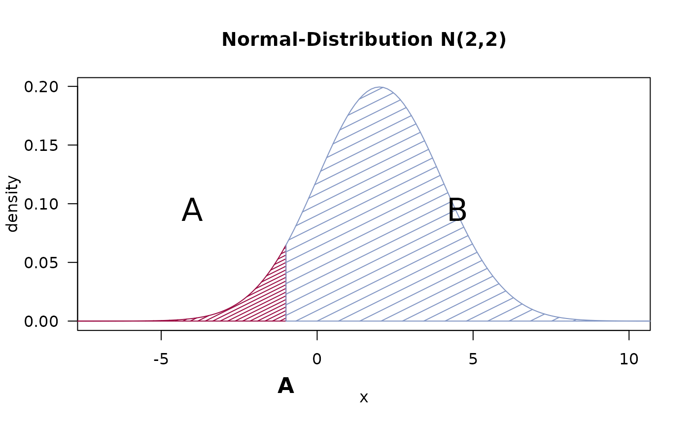
# Normal
PlotProbDist(breaks=c(-10, -1, 12), 
             function(x) dnorm(x, mean=2, sd=2), 
             blab="A", xlim=c(-7,10),
             main="Normal-Distribution N(2,2)",
             col=c(DescTools::hred, DescTools::hblue), density=c(20, 7))


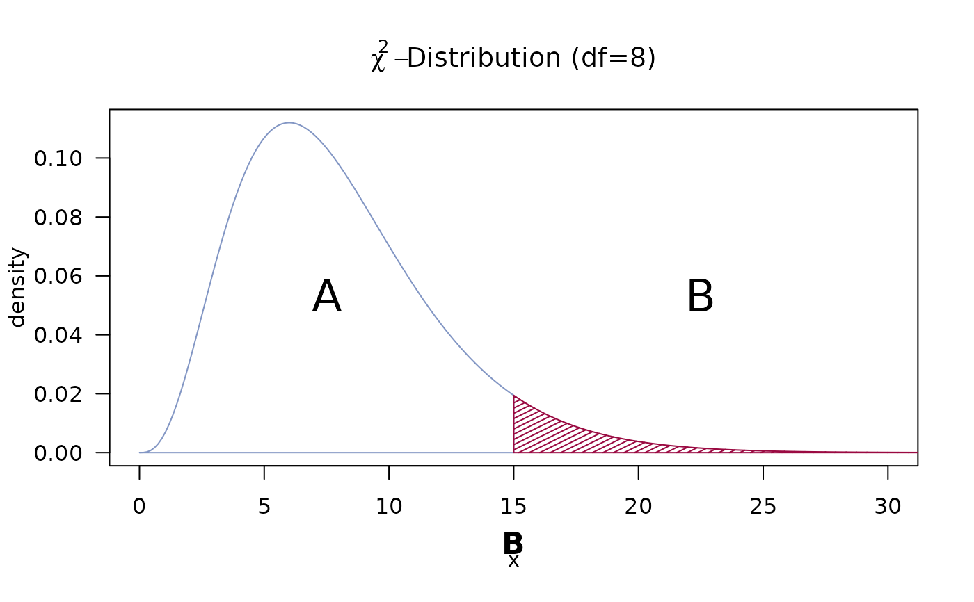
# same for Chi-square
PlotProbDist(breaks=c(0, 15, 35), 
             function(x) dchisq(x, df=8), 
             blab="B", xlim=c(0, 30),
             main=expression(paste(chi^2-Distribution, " (df=8)")),
             col=c(DescTools::hblue, DescTools::hred), density=c(0, 20))