Produce summaries of various types of variables. Calculate descriptive statistics for x and use Word as reporting tool for the numeric results and for descriptive plots. The appropriate statistics are chosen depending on the class of x. The general intention is to simplify the description process for lazy typers and return a quick, but rich summary.
Desc(x, ..., main = NULL, plotit = NULL, wrd = NULL)

# S3 method for class 'numeric'
Desc(
  x,
  main = NULL,
  maxrows = NULL,
  plotit = NULL,
  sep = NULL,
  digits = NULL,
  ...
)

# S3 method for class 'integer'
Desc(
  x,
  main = NULL,
  maxrows = NULL,
  plotit = NULL,
  sep = NULL,
  digits = NULL,
  ...
)

# S3 method for class 'factor'
Desc(
  x,
  main = NULL,
  maxrows = NULL,
  ord = NULL,
  plotit = NULL,
  sep = NULL,
  digits = NULL,
  ...
)

# S3 method for class 'labelled'
Desc(
  x,
  main = NULL,
  maxrows = NULL,
  ord = NULL,
  plotit = NULL,
  sep = NULL,
  digits = NULL,
  ...
)

# S3 method for class 'ordered'
Desc(
  x,
  main = NULL,
  maxrows = NULL,
  ord = NULL,
  plotit = NULL,
  sep = NULL,
  digits = NULL,
  ...
)

# S3 method for class 'character'
Desc(
  x,
  main = NULL,
  maxrows = NULL,
  ord = NULL,
  plotit = NULL,
  sep = NULL,
  digits = NULL,
  ...
)

# S3 method for class 'ts'
Desc(x, main = NULL, plotit = NULL, sep = NULL, digits = NULL, ...)

# S3 method for class 'logical'
Desc(
  x,
  main = NULL,
  ord = NULL,
  conf.level = 0.95,
  plotit = NULL,
  sep = NULL,
  digits = NULL,
  ...
)

# S3 method for class 'Date'
Desc(
  x,
  main = NULL,
  dprobs = NULL,
  mprobs = NULL,
  plotit = NULL,
  sep = NULL,
  digits = NULL,
  ...
)

# S3 method for class 'table'
Desc(
  x,
  main = NULL,
  conf.level = 0.95,
  verbose = 2,
  rfrq = "111",
  margins = c(1, 2),
  plotit = NULL,
  sep = NULL,
  digits = NULL,
  ...
)

# Default S3 method
Desc(
  x,
  main = NULL,
  maxrows = NULL,
  ord = NULL,
  conf.level = 0.95,
  verbose = 2,
  rfrq = "111",
  margins = c(1, 2),
  dprobs = NULL,
  mprobs = NULL,
  plotit = NULL,
  sep = NULL,
  digits = NULL,
  ...
)

# S3 method for class 'data.frame'
Desc(x, main = NULL, plotit = NULL, enum = TRUE, sep = NULL, ...)

# S3 method for class 'list'
Desc(x, main = NULL, plotit = NULL, enum = TRUE, sep = NULL, ...)

# S3 method for class 'formula'
Desc(
  formula,
  data = parent.frame(),
  subset,
  main = NULL,
  plotit = NULL,
  digits = NULL,
  ...
)

# S3 method for class 'Desc'
print(
  x,
  digits = NULL,
  plotit = NULL,
  nolabel = FALSE,
  sep = NULL,
  nomain = FALSE,
  ...
)

# S3 method for class 'Desc'
plot(x, main = NULL, ...)

# S3 method for class 'palette'
Desc(x, ...)
Arguments
- x
the object to be described. This can be a data.frame, a list, a table or a vector of the classes: numeric, integer, factor, ordered factor, logical.
- ...
further arguments to be passed to or from other methods. For the internal default method these can include:
pa vector of probabilities of the same length of
x. An error is given if any entry ofpis negative. This argument will be passed on to chisq.test(). Default isrep(1/length(x), length(x)).add_nilogical. Indicates if the group length should be displayed in the boxplot.
smoothcharacter, either "loess" or "smooth.spline" defining the type of smoother to be used in num ~ num plots. Default is "loess" for n < 500 and "smooth.spline" otherwise.
- main
(character|
NULL|NA), the main title(s).If
NULL, the title will be composed as:variable name (class(es)),
resp. number - variable name (class(es)) if the
enumoption is set toTRUE.
Use
NAif no caption should be printed at all.
- plotit
logical. Should a plot be created? The plot type will be chosen according to the classes of variables (roughly following a numeric-numeric, numeric-categorical, categorical-categorical logic). Default can be defined by option
plotit, if it does not exist then it's set toFALSE.- wrd
the pointer to a running MS Word instance, as created by
GetNewWrd()(for a new one) or byGetCurrWrd()for an existing one. All output will then be redirected there. Default isNULL, which will report all results to the console.- maxrows
numeric; defines the maximum number of rows in a frequency table to be reported. For factors with many levels it is often not interesting to see all of them. Default is set to 12 most frequent ones (resp. the first ones if
ordis set to"levels"or"names").For a numeric argument x
maxrowsis the minimum number of unique values needed for a numeric variable to be treated as continuous. If left to its defaultNULL, x will be regarded as continuous if it has more than 12 single values. In this case the list of extreme values will be displayed and the frequency table else.If
maxrowsis < 1 it will be interpreted as percentage. In this case just as many rows, as themaxrowsmost frequent levels will be shown. Say, ifmaxrowsis set to0.8, then the number of rows is fixed so, that the highest cumulative relative frequency is the first one going beyond 0.8.Setting
maxrowstoInfwill unconditionally report all values and also produce a plot with type "h" instead of a histogram.- sep
character. The separator for the title. By default a line of
"-"for the current width of the screen(options("width"))will be used.- digits
integer. With how many digits should the relative frequencies be formatted? Default can be set by DescToolsOptions(digits=x).
- ord
character out of
"name"(alphabetical order),"level","asc"(by frequencies ascending),"desc"(by frequencies descending) defining the order for a frequency table as used for factors, numerics with few unique values and logicals. Factors (and character vectors) are by default ordered by their descending frequencies, ordered factors by their natural order.- conf.level
confidence level of the interval. If set to
NAno confidence interval will be calculated. Default is 0.95.- dprobs, mprobs
a vector with the probabilities for the Chi-Square test for days, resp. months, when describing a
Datevariable. If this is left toNULL(default) then a uniform distribution will be used for days and a monthdays distribution in a non leap year (p = c(31/365, 28/365, 31/365, ...)) for the months.
Applies only toDatesand is ignored else.- verbose
integer out of
c(2, 1, 3)defining the verbosity of the reported results. 2 (default) means medium, 1 less and 3 extensive results.
Applies only to tables and is ignored else.- rfrq
a string with 3 characters, each of them being
1or0, defining which percentages should be reported. The first position is interpreted as total percentages, the second as row percentages and the third as column percentages. "011" hence produces a table output with row and column percentages. If set toNULLrfrqis defined in dependency ofverbose(verbose = 1setsrfrqto"000"and else to"111", latter meaning all percentages will be reported.)
Applies only to tables and is ignored else.- margins
a vector, consisting out of 1 and/or 2. Defines the margin sums to be included. Row margins are reported if margins is set to 1. Set it to 2 for column margins and c(1,2) for both.
Default isNULL(none).
Applies only to tables and is ignored else.- enum
logical, determining if in data.frames and lists a sequential number should be included in the main title. Default is TRUE. The reason for this option is, that if a Word report with enumerated headings is created, the numbers may be redundant or inconsistent.
- formula
a formula of the form
lhs ~ rhswherelhsgives the data values and rhs the corresponding groups.- data
an optional matrix or data frame containing the variables in the formula
formula. By default the variables are taken fromenvironment(formula).- subset
an optional vector specifying a subset of observations to be used.
- nolabel
logical, defining if labels (defined as attribute with the name
label, as done byLabel) should be plotted.- nomain
logical, determines if the main title of the output is printed or not, default is
TRUE.
Value
A list containing the following components:
- length
the length of the vector (n + NAs).
- n
the valid entries (NAs are excluded)
- NAs
number of NAs
- unique
number of unique values.
- 0s
number of zeros
- mean
arithmetic mean
- MeanSE
standard error of the mean, as calculated by
MeanSE().- quant
a table of quantiles, as calculated by quantile(x, probs = c(.05,.10,.25,.5,.75,.9,.95), na.rm = TRUE).
- sd
standard deviation
- vcoef
coefficient of variation:
mean(x)/sd(x).- mad
median absolute deviation (
stats::mad()).- IQR
interquartile range
- skew
skewness, as calculated by
Skew().- kurt
kurtosis, as calculated by
Kurt().- highlow
the lowest and the highest values, reported with their frequencies in brackets, if > 1.
- frq
a data.frame of absolute and relative frequencies given by
Freq()ifmaxlevels> unique values in the vector.
Details
A 2-dimensional table will be described with it's relative frequencies, a
short summary containing the total cases, the dimensions of the table,
chi-square tests and some association measures as phi-coefficient,
contingency coefficient and Cramer's V.
Tables with higher dimensions will simply be printed as flat table,
with marginal sums for the first and for the last dimension.
Desc is a generic function. It dispatches to one of the methods above
depending on the class of its first argument. Typing ?Desc + TAB at the
prompt should present a choice of links: the help pages for each of these
Desc methods (at least if you're using RStudio, which anyway is
recommended). You don't need to use the full name of the method although you
may if you wish; i.e., Desc(x) is idiomatic R but you can bypass method
dispatch by going direct if you wish: Desc.numeric(x).
This function produces a rich description of a factor, containing length,
number of NAs, number of levels and detailed frequencies of all levels. The
order of the frequency table can be chosen between descending/ascending
frequency, labels or levels. For ordered factors the order default is
"level". Character vectors are treated as unordered factors Desc.char
converts x to a factor an processes x as factor.
Desc.ordered does nothing more than changing the standard order for the
frequencies to it's intrinsic order, which means order "level"
instead of "desc" in the factor case.
Description interface for dates. We do here what seems reasonable for describing dates. We start with a short summary about length, number of NAs and extreme values, before we describe the frequencies of the weekdays and months, rounded up by a chi-square test.
A 2-dimensional table will be described with it's relative frequencies, a
short summary containing the total cases, the dimensions of the table,
chi-square tests and some association measures as phi-coefficient,
contingency coefficient and Cramer's V.
Tables with higher dimensions will simply be printed as flat table,
with marginal sums for the first and for the last dimension.
Note that NAs cannot be handled by this interface, as tables in general come
in "as.is", say basically as a matrix without any further information about
potentially previously cleared NAs.
Description of a dichotomous variable. This can either be a logical vector,
a factor with two levels or a numeric variable with only two unique values.
The confidence levels for the relative frequencies are calculated by
BinomCI(), method "Wilson" on a confidence level defined
by conf.level. Dichotomous variables can easily be condensed in one
graphical representation. Desc for a set of flags (=dichotomous variables)
calculates the frequencies, a binomial confidence interval and produces a
kind of dotplot with error bars. Motivation for this function is, that
dichotomous variable in general do not contain intense information.
Therefore it makes sense to condense the description of sets of dichotomous
variables.
The formula interface accepts the formula operators +, :,
*, I(), 1 and evaluates any function. The left hand
side and right hand side of the formula are evaluated the same way. The
variable pairs are processed in dependency of their classes.
Word This function is not thought of being directly run by the end user.
It will normally be called automatically, when a pointer to a Word instance
is passed to the function Desc().
However DescWrd takes
some more specific arguments concerning the Word output (like font or
fontsize), which can make it necessary to call the function directly.
See also
Other Statistical summary functions:
Abstract()
Examples
opt <- DescToolsOptions()
# implemented classes:
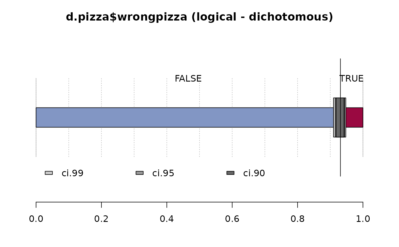
Desc(d.pizza$wrongpizza) # logical
#> ──────────────────────────────────────────────────────────────────────────────
#> d.pizza$wrongpizza (logical - dichotomous)
#>
#> length n NAs unique
#> 1'209 1'205 4 2
#> 99.7% 0.3%
#>
#> freq perc lci.95 uci.95'
#> FALSE 1'122 93.1% 91.5% 94.4%
#> TRUE 83 6.9% 5.6% 8.5%
#>
#> ' 95%-CI (Wilson)
#>
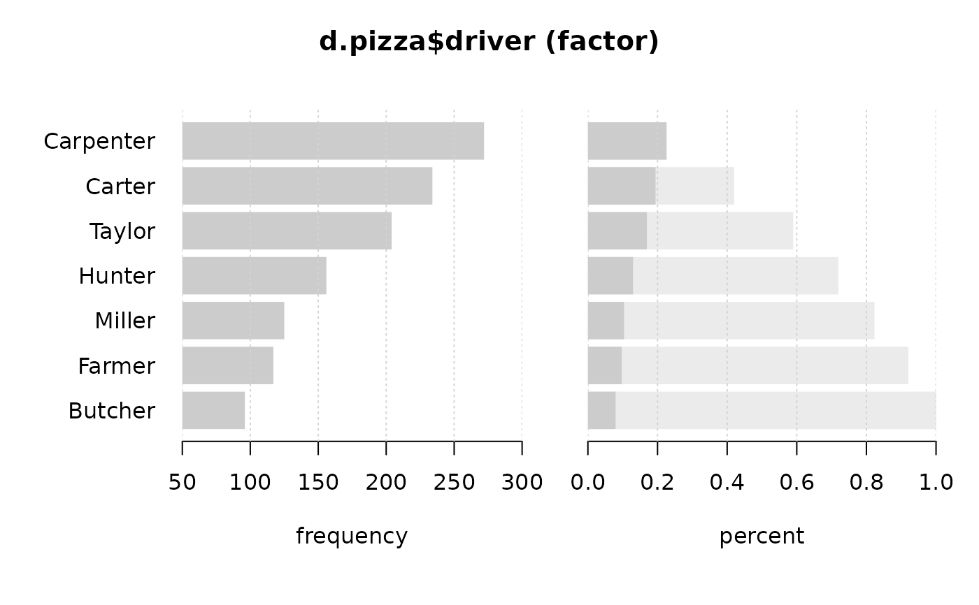
 Desc(d.pizza$driver) # factor
#> ──────────────────────────────────────────────────────────────────────────────
#> d.pizza$driver (factor)
#>
#> length n NAs unique levels dupes
#> 1'209 1'204 5 7 7 y
#> 99.6% 0.4%
#>
#> level freq perc cumfreq cumperc
#> 1 Carpenter 272 22.6% 272 22.6%
#> 2 Carter 234 19.4% 506 42.0%
#> 3 Taylor 204 16.9% 710 59.0%
#> 4 Hunter 156 13.0% 866 71.9%
#> 5 Miller 125 10.4% 991 82.3%
#> 6 Farmer 117 9.7% 1'108 92.0%
#> 7 Butcher 96 8.0% 1'204 100.0%
#>
Desc(d.pizza$driver) # factor
#> ──────────────────────────────────────────────────────────────────────────────
#> d.pizza$driver (factor)
#>
#> length n NAs unique levels dupes
#> 1'209 1'204 5 7 7 y
#> 99.6% 0.4%
#>
#> level freq perc cumfreq cumperc
#> 1 Carpenter 272 22.6% 272 22.6%
#> 2 Carter 234 19.4% 506 42.0%
#> 3 Taylor 204 16.9% 710 59.0%
#> 4 Hunter 156 13.0% 866 71.9%
#> 5 Miller 125 10.4% 991 82.3%
#> 6 Farmer 117 9.7% 1'108 92.0%
#> 7 Butcher 96 8.0% 1'204 100.0%
#>
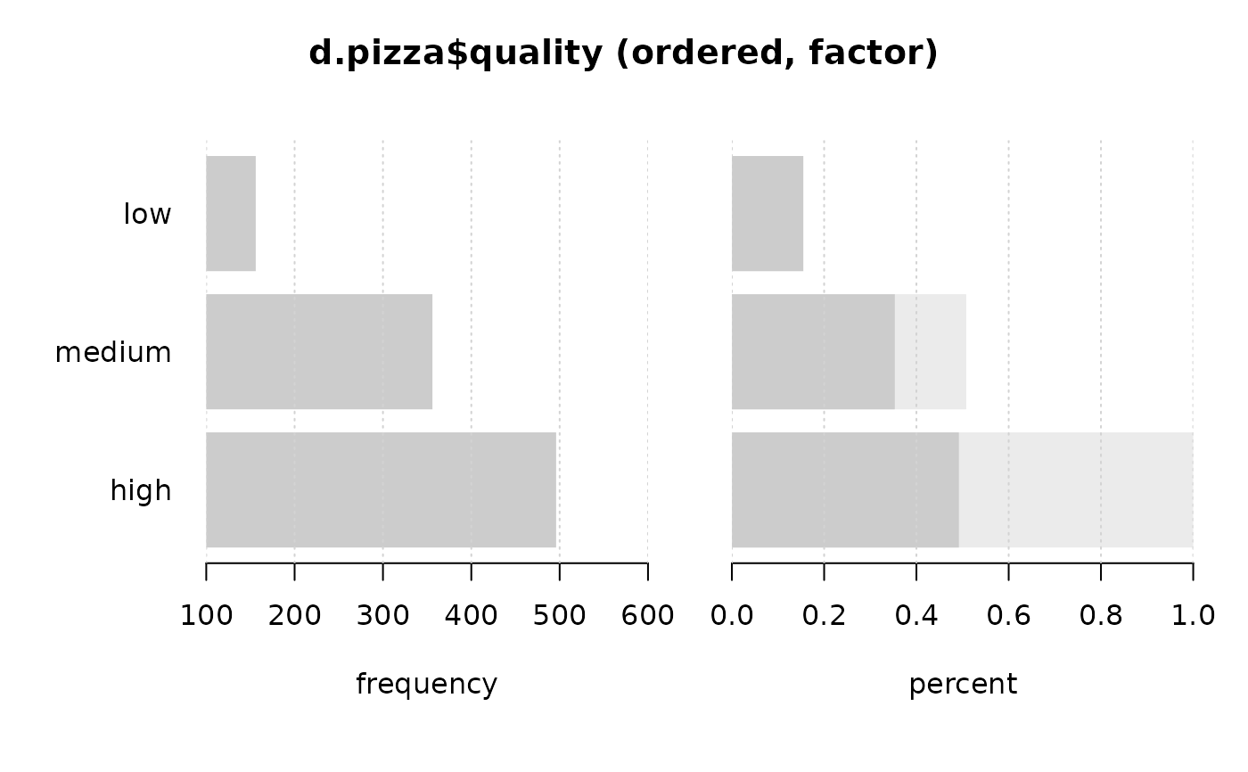
 Desc(d.pizza$quality) # ordered factor
#> ──────────────────────────────────────────────────────────────────────────────
#> d.pizza$quality (ordered, factor)
#>
#> length n NAs unique levels dupes
#> 1'209 1'008 201 3 3 y
#> 83.4% 16.6%
#>
#> level freq perc cumfreq cumperc
#> 1 low 156 15.5% 156 15.5%
#> 2 medium 356 35.3% 512 50.8%
#> 3 high 496 49.2% 1'008 100.0%
#>
Desc(d.pizza$quality) # ordered factor
#> ──────────────────────────────────────────────────────────────────────────────
#> d.pizza$quality (ordered, factor)
#>
#> length n NAs unique levels dupes
#> 1'209 1'008 201 3 3 y
#> 83.4% 16.6%
#>
#> level freq perc cumfreq cumperc
#> 1 low 156 15.5% 156 15.5%
#> 2 medium 356 35.3% 512 50.8%
#> 3 high 496 49.2% 1'008 100.0%
#>
 Desc(as.character(d.pizza$driver)) # character
#> ──────────────────────────────────────────────────────────────────────────────
#> as.character(d.pizza$driver) (character)
#>
#> length n NAs unique levels dupes
#> 1'209 1'204 5 7 7 y
#> 99.6% 0.4%
#>
#> level freq perc cumfreq cumperc
#> 1 Carpenter 272 22.6% 272 22.6%
#> 2 Carter 234 19.4% 506 42.0%
#> 3 Taylor 204 16.9% 710 59.0%
#> 4 Hunter 156 13.0% 866 71.9%
#> 5 Miller 125 10.4% 991 82.3%
#> 6 Farmer 117 9.7% 1'108 92.0%
#> 7 Butcher 96 8.0% 1'204 100.0%
#>
Desc(as.character(d.pizza$driver)) # character
#> ──────────────────────────────────────────────────────────────────────────────
#> as.character(d.pizza$driver) (character)
#>
#> length n NAs unique levels dupes
#> 1'209 1'204 5 7 7 y
#> 99.6% 0.4%
#>
#> level freq perc cumfreq cumperc
#> 1 Carpenter 272 22.6% 272 22.6%
#> 2 Carter 234 19.4% 506 42.0%
#> 3 Taylor 204 16.9% 710 59.0%
#> 4 Hunter 156 13.0% 866 71.9%
#> 5 Miller 125 10.4% 991 82.3%
#> 6 Farmer 117 9.7% 1'108 92.0%
#> 7 Butcher 96 8.0% 1'204 100.0%
#>
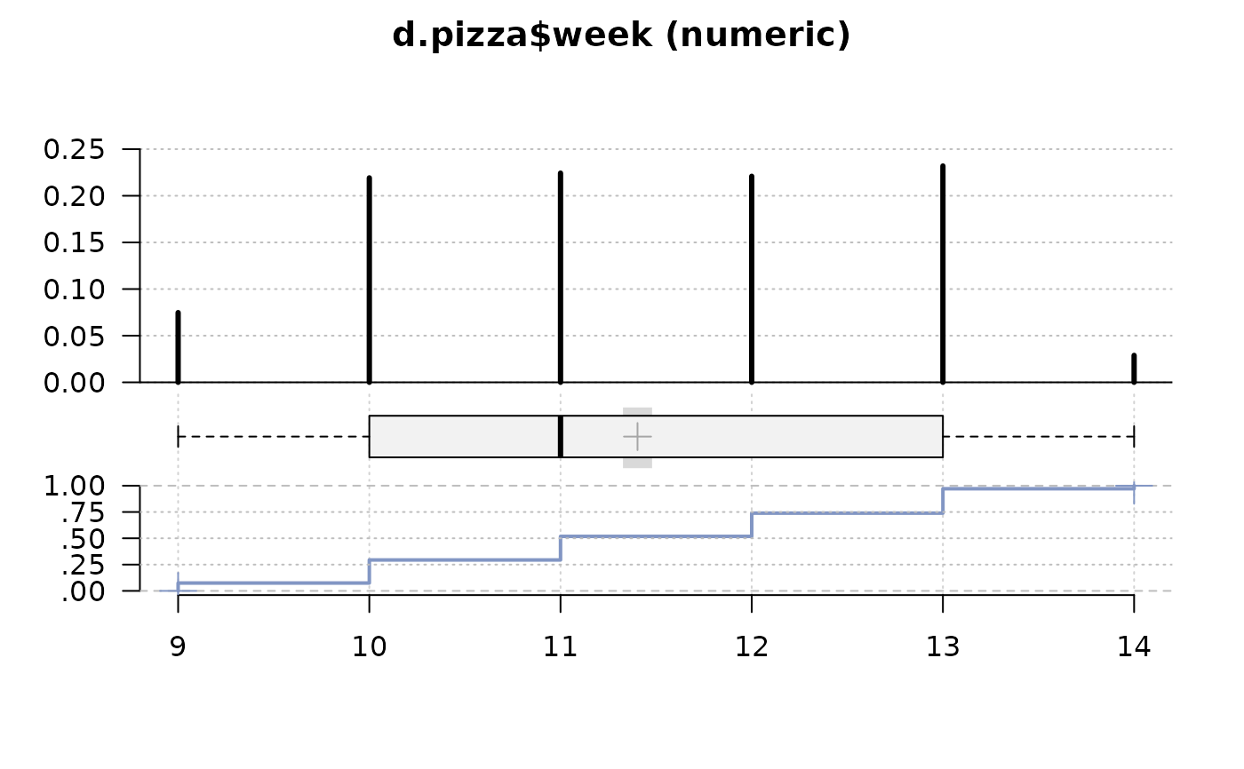
 Desc(d.pizza$week) # integer
#> ──────────────────────────────────────────────────────────────────────────────
#> d.pizza$week (numeric)
#>
#> length n NAs unique 0s mean meanCI'
#> 1'209 1'177 32 6 0 11.40 11.33
#> 97.4% 2.6% 0.0% 11.48
#>
#> .05 .10 .25 median .75 .90 .95
#> 9.00 10.00 10.00 11.00 13.00 13.00 13.00
#>
#> range sd vcoef mad IQR skew kurt
#> 5.00 1.33 0.12 1.48 3.00 -0.07 -1.01
#>
#>
#> value freq perc cumfreq cumperc
#> 1 9 88 7.5% 88 7.5%
#> 2 10 258 21.9% 346 29.4%
#> 3 11 264 22.4% 610 51.8%
#> 4 12 260 22.1% 870 73.9%
#> 5 13 273 23.2% 1'143 97.1%
#> 6 14 34 2.9% 1'177 100.0%
#>
#> ' 95%-CI (classic)
#>
Desc(d.pizza$week) # integer
#> ──────────────────────────────────────────────────────────────────────────────
#> d.pizza$week (numeric)
#>
#> length n NAs unique 0s mean meanCI'
#> 1'209 1'177 32 6 0 11.40 11.33
#> 97.4% 2.6% 0.0% 11.48
#>
#> .05 .10 .25 median .75 .90 .95
#> 9.00 10.00 10.00 11.00 13.00 13.00 13.00
#>
#> range sd vcoef mad IQR skew kurt
#> 5.00 1.33 0.12 1.48 3.00 -0.07 -1.01
#>
#>
#> value freq perc cumfreq cumperc
#> 1 9 88 7.5% 88 7.5%
#> 2 10 258 21.9% 346 29.4%
#> 3 11 264 22.4% 610 51.8%
#> 4 12 260 22.1% 870 73.9%
#> 5 13 273 23.2% 1'143 97.1%
#> 6 14 34 2.9% 1'177 100.0%
#>
#> ' 95%-CI (classic)
#>
 Desc(d.pizza$delivery_min) # numeric
#> ──────────────────────────────────────────────────────────────────────────────
#> d.pizza$delivery_min (numeric)
#>
#> length n NAs unique 0s mean meanCI'
#> 1'209 1'209 0 384 0 25.65 25.04
#> 100.0% 0.0% 0.0% 26.26
#>
#> .05 .10 .25 median .75 .90 .95
#> 10.40 11.60 17.40 24.40 32.50 40.42 45.20
#>
#> range sd vcoef mad IQR skew kurt
#> 56.80 10.84 0.42 11.27 15.10 0.61 0.10
#>
#> lowest : 8.8 (3), 8.9, 9.0 (3), 9.1 (5), 9.2 (3)
#> highest: 61.9, 62.7, 62.9, 63.2, 65.6
#>
#> ' 95%-CI (classic)
#>
Desc(d.pizza$delivery_min) # numeric
#> ──────────────────────────────────────────────────────────────────────────────
#> d.pizza$delivery_min (numeric)
#>
#> length n NAs unique 0s mean meanCI'
#> 1'209 1'209 0 384 0 25.65 25.04
#> 100.0% 0.0% 0.0% 26.26
#>
#> .05 .10 .25 median .75 .90 .95
#> 10.40 11.60 17.40 24.40 32.50 40.42 45.20
#>
#> range sd vcoef mad IQR skew kurt
#> 56.80 10.84 0.42 11.27 15.10 0.61 0.10
#>
#> lowest : 8.8 (3), 8.9, 9.0 (3), 9.1 (5), 9.2 (3)
#> highest: 61.9, 62.7, 62.9, 63.2, 65.6
#>
#> ' 95%-CI (classic)
#>
 Desc(d.pizza$date) # Date
#> ──────────────────────────────────────────────────────────────────────────────
#> d.pizza$date (Date)
#>
#> length n NAs unique
#> 1'209 1'177 32 31
#> 97.4% 2.6%
#>
#> lowest : 2014-03-01 (42), 2014-03-02 (46), 2014-03-03 (26), 2014-03-04 (19)
#> highest: 2014-03-28 (46), 2014-03-29 (53), 2014-03-30 (43), 2014-03-31 (34)
#>
#>
#> Weekday:
#>
#> Pearson's Chi-squared test (1-dim uniform):
#> X-squared = 78.879, df = 6, p-value = 6.09e-15
#>
#> level freq perc cumfreq cumperc
#> 1 Monday 144 12.2% 144 12.2%
#> 2 Tuesday 117 9.9% 261 22.2%
#> 3 Wednesday 134 11.4% 395 33.6%
#> 4 Thursday 147 12.5% 542 46.0%
#> 5 Friday 171 14.5% 713 60.6%
#> 6 Saturday 244 20.7% 957 81.3%
#> 7 Sunday 220 18.7% 1'177 100.0%
#>
#> Months:
#>
#> Pearson's Chi-squared test (1-dim uniform):
#> X-squared = 12947, df = 11, p-value < 2.2e-16
#>
#> level freq perc cumfreq cumperc
#> 1 January 0 0.0% 0 0.0%
#> 2 February 0 0.0% 0 0.0%
#> 3 March 1'177 100.0% 1'177 100.0%
#> 4 April 0 0.0% 1'177 100.0%
#> 5 May 0 0.0% 1'177 100.0%
#> 6 June 0 0.0% 1'177 100.0%
#> 7 July 0 0.0% 1'177 100.0%
#> 8 August 0 0.0% 1'177 100.0%
#> 9 September 0 0.0% 1'177 100.0%
#> 10 October 0 0.0% 1'177 100.0%
#> 11 November 0 0.0% 1'177 100.0%
#> 12 December 0 0.0% 1'177 100.0%
#>
#> By days :
#>
#> level freq perc cumfreq cumperc
#> 1 2014-03-01 42 3.6% 42 3.6%
#> 2 2014-03-02 46 3.9% 88 7.5%
#> 3 2014-03-03 26 2.2% 114 9.7%
#> 4 2014-03-04 19 1.6% 133 11.3%
#> 5 2014-03-05 33 2.8% 166 14.1%
#> 6 2014-03-06 39 3.3% 205 17.4%
#> 7 2014-03-07 44 3.7% 249 21.2%
#> 8 2014-03-08 55 4.7% 304 25.8%
#> 9 2014-03-09 42 3.6% 346 29.4%
#> 10 2014-03-10 26 2.2% 372 31.6%
#> 11 2014-03-11 34 2.9% 406 34.5%
#> 12 2014-03-12 36 3.1% 442 37.6%
#> 13 2014-03-13 35 3.0% 477 40.5%
#> 14 2014-03-14 38 3.2% 515 43.8%
#> 15 2014-03-15 48 4.1% 563 47.8%
#> 16 2014-03-16 47 4.0% 610 51.8%
#> 17 2014-03-17 30 2.5% 640 54.4%
#> 18 2014-03-18 32 2.7% 672 57.1%
#> 19 2014-03-19 31 2.6% 703 59.7%
#> 20 2014-03-20 36 3.1% 739 62.8%
#> 21 2014-03-21 43 3.7% 782 66.4%
#> 22 2014-03-22 46 3.9% 828 70.3%
#> 23 2014-03-23 42 3.6% 870 73.9%
#> 24 2014-03-24 28 2.4% 898 76.3%
#> 25 2014-03-25 32 2.7% 930 79.0%
#> 26 2014-03-26 34 2.9% 964 81.9%
#> 27 2014-03-27 37 3.1% 1'001 85.0%
#> 28 2014-03-28 46 3.9% 1'047 89.0%
#> 29 2014-03-29 53 4.5% 1'100 93.5%
#> 30 2014-03-30 43 3.7% 1'143 97.1%
#> 31 2014-03-31 34 2.9% 1'177 100.0%
#>
Desc(d.pizza$date) # Date
#> ──────────────────────────────────────────────────────────────────────────────
#> d.pizza$date (Date)
#>
#> length n NAs unique
#> 1'209 1'177 32 31
#> 97.4% 2.6%
#>
#> lowest : 2014-03-01 (42), 2014-03-02 (46), 2014-03-03 (26), 2014-03-04 (19)
#> highest: 2014-03-28 (46), 2014-03-29 (53), 2014-03-30 (43), 2014-03-31 (34)
#>
#>
#> Weekday:
#>
#> Pearson's Chi-squared test (1-dim uniform):
#> X-squared = 78.879, df = 6, p-value = 6.09e-15
#>
#> level freq perc cumfreq cumperc
#> 1 Monday 144 12.2% 144 12.2%
#> 2 Tuesday 117 9.9% 261 22.2%
#> 3 Wednesday 134 11.4% 395 33.6%
#> 4 Thursday 147 12.5% 542 46.0%
#> 5 Friday 171 14.5% 713 60.6%
#> 6 Saturday 244 20.7% 957 81.3%
#> 7 Sunday 220 18.7% 1'177 100.0%
#>
#> Months:
#>
#> Pearson's Chi-squared test (1-dim uniform):
#> X-squared = 12947, df = 11, p-value < 2.2e-16
#>
#> level freq perc cumfreq cumperc
#> 1 January 0 0.0% 0 0.0%
#> 2 February 0 0.0% 0 0.0%
#> 3 March 1'177 100.0% 1'177 100.0%
#> 4 April 0 0.0% 1'177 100.0%
#> 5 May 0 0.0% 1'177 100.0%
#> 6 June 0 0.0% 1'177 100.0%
#> 7 July 0 0.0% 1'177 100.0%
#> 8 August 0 0.0% 1'177 100.0%
#> 9 September 0 0.0% 1'177 100.0%
#> 10 October 0 0.0% 1'177 100.0%
#> 11 November 0 0.0% 1'177 100.0%
#> 12 December 0 0.0% 1'177 100.0%
#>
#> By days :
#>
#> level freq perc cumfreq cumperc
#> 1 2014-03-01 42 3.6% 42 3.6%
#> 2 2014-03-02 46 3.9% 88 7.5%
#> 3 2014-03-03 26 2.2% 114 9.7%
#> 4 2014-03-04 19 1.6% 133 11.3%
#> 5 2014-03-05 33 2.8% 166 14.1%
#> 6 2014-03-06 39 3.3% 205 17.4%
#> 7 2014-03-07 44 3.7% 249 21.2%
#> 8 2014-03-08 55 4.7% 304 25.8%
#> 9 2014-03-09 42 3.6% 346 29.4%
#> 10 2014-03-10 26 2.2% 372 31.6%
#> 11 2014-03-11 34 2.9% 406 34.5%
#> 12 2014-03-12 36 3.1% 442 37.6%
#> 13 2014-03-13 35 3.0% 477 40.5%
#> 14 2014-03-14 38 3.2% 515 43.8%
#> 15 2014-03-15 48 4.1% 563 47.8%
#> 16 2014-03-16 47 4.0% 610 51.8%
#> 17 2014-03-17 30 2.5% 640 54.4%
#> 18 2014-03-18 32 2.7% 672 57.1%
#> 19 2014-03-19 31 2.6% 703 59.7%
#> 20 2014-03-20 36 3.1% 739 62.8%
#> 21 2014-03-21 43 3.7% 782 66.4%
#> 22 2014-03-22 46 3.9% 828 70.3%
#> 23 2014-03-23 42 3.6% 870 73.9%
#> 24 2014-03-24 28 2.4% 898 76.3%
#> 25 2014-03-25 32 2.7% 930 79.0%
#> 26 2014-03-26 34 2.9% 964 81.9%
#> 27 2014-03-27 37 3.1% 1'001 85.0%
#> 28 2014-03-28 46 3.9% 1'047 89.0%
#> 29 2014-03-29 53 4.5% 1'100 93.5%
#> 30 2014-03-30 43 3.7% 1'143 97.1%
#> 31 2014-03-31 34 2.9% 1'177 100.0%
#>


 Desc(d.pizza)
#> ──────────────────────────────────────────────────────────────────────────────
#> Describe d.pizza (data.frame):
#>
#> data frame: 1209 obs. of 16 variables
#> 917 complete cases (75.8%)
#>
#> Nr Class ColName NAs Levels
#> 1 int index .
#> 2 dat date 32 (2.6%)
#> 3 num week 32 (2.6%)
#> 4 num weekday 32 (2.6%)
#> 5 fac area 10 (0.8%) (3): 1-Brent, 2-Camden,
#> 3-Westminster
#> 6 int count 12 (1.0%)
#> 7 log rabate 12 (1.0%)
#> 8 num price 12 (1.0%)
#> 9 fac operator 8 (0.7%) (3): 1-Allanah, 2-Maria, 3-Rhonda
#> 10 fac driver 5 (0.4%) (7): 1-Butcher, 2-Carpenter,
#> 3-Carter, 4-Farmer, 5-Hunter, ...
#> 11 num delivery_min .
#> 12 num temperature 39 (3.2%)
#> 13 int wine_ordered 12 (1.0%)
#> 14 int wine_delivered 12 (1.0%)
#> 15 log wrongpizza 4 (0.3%)
#> 16 ord quality 201 (16.6%) (3): 1-low, 2-medium, 3-high
#>
#>
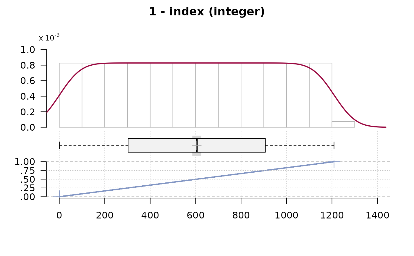
#> ──────────────────────────────────────────────────────────────────────────────
#> 1 - index (integer)
#>
#> length n NAs unique 0s mean meanCI'
#> 1'209 1'209 0 = n 0 605.00 585.30
#> 100.0% 0.0% 0.0% 624.70
#>
#> .05 .10 .25 median .75 .90 .95
#> 61.40 121.80 303.00 605.00 907.00 1'088.20 1'148.60
#>
#> range sd vcoef mad IQR skew kurt
#> 1'208.00 349.15 0.58 447.75 604.00 0.00 -1.20
#>
#> lowest : 1, 2, 3, 4, 5
#> highest: 1'205, 1'206, 1'207, 1'208, 1'209
#>
#> ' 95%-CI (classic)
#>
Desc(d.pizza)
#> ──────────────────────────────────────────────────────────────────────────────
#> Describe d.pizza (data.frame):
#>
#> data frame: 1209 obs. of 16 variables
#> 917 complete cases (75.8%)
#>
#> Nr Class ColName NAs Levels
#> 1 int index .
#> 2 dat date 32 (2.6%)
#> 3 num week 32 (2.6%)
#> 4 num weekday 32 (2.6%)
#> 5 fac area 10 (0.8%) (3): 1-Brent, 2-Camden,
#> 3-Westminster
#> 6 int count 12 (1.0%)
#> 7 log rabate 12 (1.0%)
#> 8 num price 12 (1.0%)
#> 9 fac operator 8 (0.7%) (3): 1-Allanah, 2-Maria, 3-Rhonda
#> 10 fac driver 5 (0.4%) (7): 1-Butcher, 2-Carpenter,
#> 3-Carter, 4-Farmer, 5-Hunter, ...
#> 11 num delivery_min .
#> 12 num temperature 39 (3.2%)
#> 13 int wine_ordered 12 (1.0%)
#> 14 int wine_delivered 12 (1.0%)
#> 15 log wrongpizza 4 (0.3%)
#> 16 ord quality 201 (16.6%) (3): 1-low, 2-medium, 3-high
#>
#>
#> ──────────────────────────────────────────────────────────────────────────────
#> 1 - index (integer)
#>
#> length n NAs unique 0s mean meanCI'
#> 1'209 1'209 0 = n 0 605.00 585.30
#> 100.0% 0.0% 0.0% 624.70
#>
#> .05 .10 .25 median .75 .90 .95
#> 61.40 121.80 303.00 605.00 907.00 1'088.20 1'148.60
#>
#> range sd vcoef mad IQR skew kurt
#> 1'208.00 349.15 0.58 447.75 604.00 0.00 -1.20
#>
#> lowest : 1, 2, 3, 4, 5
#> highest: 1'205, 1'206, 1'207, 1'208, 1'209
#>
#> ' 95%-CI (classic)
#>
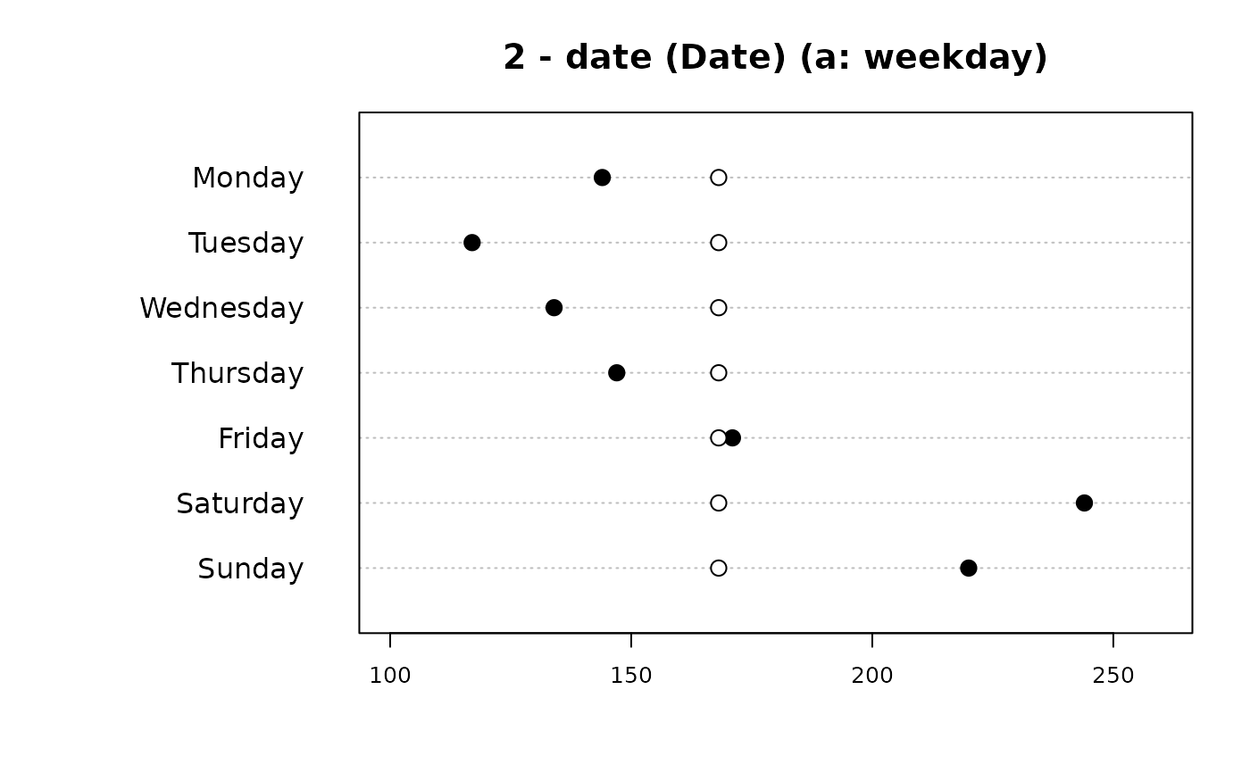
 #> ──────────────────────────────────────────────────────────────────────────────
#> 2 - date (Date)
#>
#> length n NAs unique
#> 1'209 1'177 32 31
#> 97.4% 2.6%
#>
#> lowest : 2014-03-01 (42), 2014-03-02 (46), 2014-03-03 (26), 2014-03-04 (19)
#> highest: 2014-03-28 (46), 2014-03-29 (53), 2014-03-30 (43), 2014-03-31 (34)
#>
#>
#> Weekday:
#>
#> Pearson's Chi-squared test (1-dim uniform):
#> X-squared = 78.879, df = 6, p-value = 6.09e-15
#>
#> level freq perc cumfreq cumperc
#> 1 Monday 144 12.2% 144 12.2%
#> 2 Tuesday 117 9.9% 261 22.2%
#> 3 Wednesday 134 11.4% 395 33.6%
#> 4 Thursday 147 12.5% 542 46.0%
#> 5 Friday 171 14.5% 713 60.6%
#> 6 Saturday 244 20.7% 957 81.3%
#> 7 Sunday 220 18.7% 1'177 100.0%
#>
#> Months:
#>
#> Pearson's Chi-squared test (1-dim uniform):
#> X-squared = 12947, df = 11, p-value < 2.2e-16
#>
#> level freq perc cumfreq cumperc
#> 1 January 0 0.0% 0 0.0%
#> 2 February 0 0.0% 0 0.0%
#> 3 March 1'177 100.0% 1'177 100.0%
#> 4 April 0 0.0% 1'177 100.0%
#> 5 May 0 0.0% 1'177 100.0%
#> 6 June 0 0.0% 1'177 100.0%
#> 7 July 0 0.0% 1'177 100.0%
#> 8 August 0 0.0% 1'177 100.0%
#> 9 September 0 0.0% 1'177 100.0%
#> 10 October 0 0.0% 1'177 100.0%
#> 11 November 0 0.0% 1'177 100.0%
#> 12 December 0 0.0% 1'177 100.0%
#>
#> By days :
#>
#> level freq perc cumfreq cumperc
#> 1 2014-03-01 42 3.6% 42 3.6%
#> 2 2014-03-02 46 3.9% 88 7.5%
#> 3 2014-03-03 26 2.2% 114 9.7%
#> 4 2014-03-04 19 1.6% 133 11.3%
#> 5 2014-03-05 33 2.8% 166 14.1%
#> 6 2014-03-06 39 3.3% 205 17.4%
#> 7 2014-03-07 44 3.7% 249 21.2%
#> 8 2014-03-08 55 4.7% 304 25.8%
#> 9 2014-03-09 42 3.6% 346 29.4%
#> 10 2014-03-10 26 2.2% 372 31.6%
#> 11 2014-03-11 34 2.9% 406 34.5%
#> 12 2014-03-12 36 3.1% 442 37.6%
#> 13 2014-03-13 35 3.0% 477 40.5%
#> 14 2014-03-14 38 3.2% 515 43.8%
#> 15 2014-03-15 48 4.1% 563 47.8%
#> 16 2014-03-16 47 4.0% 610 51.8%
#> 17 2014-03-17 30 2.5% 640 54.4%
#> 18 2014-03-18 32 2.7% 672 57.1%
#> 19 2014-03-19 31 2.6% 703 59.7%
#> 20 2014-03-20 36 3.1% 739 62.8%
#> 21 2014-03-21 43 3.7% 782 66.4%
#> 22 2014-03-22 46 3.9% 828 70.3%
#> 23 2014-03-23 42 3.6% 870 73.9%
#> 24 2014-03-24 28 2.4% 898 76.3%
#> 25 2014-03-25 32 2.7% 930 79.0%
#> 26 2014-03-26 34 2.9% 964 81.9%
#> 27 2014-03-27 37 3.1% 1'001 85.0%
#> 28 2014-03-28 46 3.9% 1'047 89.0%
#> 29 2014-03-29 53 4.5% 1'100 93.5%
#> 30 2014-03-30 43 3.7% 1'143 97.1%
#> 31 2014-03-31 34 2.9% 1'177 100.0%
#>
#> ──────────────────────────────────────────────────────────────────────────────
#> 2 - date (Date)
#>
#> length n NAs unique
#> 1'209 1'177 32 31
#> 97.4% 2.6%
#>
#> lowest : 2014-03-01 (42), 2014-03-02 (46), 2014-03-03 (26), 2014-03-04 (19)
#> highest: 2014-03-28 (46), 2014-03-29 (53), 2014-03-30 (43), 2014-03-31 (34)
#>
#>
#> Weekday:
#>
#> Pearson's Chi-squared test (1-dim uniform):
#> X-squared = 78.879, df = 6, p-value = 6.09e-15
#>
#> level freq perc cumfreq cumperc
#> 1 Monday 144 12.2% 144 12.2%
#> 2 Tuesday 117 9.9% 261 22.2%
#> 3 Wednesday 134 11.4% 395 33.6%
#> 4 Thursday 147 12.5% 542 46.0%
#> 5 Friday 171 14.5% 713 60.6%
#> 6 Saturday 244 20.7% 957 81.3%
#> 7 Sunday 220 18.7% 1'177 100.0%
#>
#> Months:
#>
#> Pearson's Chi-squared test (1-dim uniform):
#> X-squared = 12947, df = 11, p-value < 2.2e-16
#>
#> level freq perc cumfreq cumperc
#> 1 January 0 0.0% 0 0.0%
#> 2 February 0 0.0% 0 0.0%
#> 3 March 1'177 100.0% 1'177 100.0%
#> 4 April 0 0.0% 1'177 100.0%
#> 5 May 0 0.0% 1'177 100.0%
#> 6 June 0 0.0% 1'177 100.0%
#> 7 July 0 0.0% 1'177 100.0%
#> 8 August 0 0.0% 1'177 100.0%
#> 9 September 0 0.0% 1'177 100.0%
#> 10 October 0 0.0% 1'177 100.0%
#> 11 November 0 0.0% 1'177 100.0%
#> 12 December 0 0.0% 1'177 100.0%
#>
#> By days :
#>
#> level freq perc cumfreq cumperc
#> 1 2014-03-01 42 3.6% 42 3.6%
#> 2 2014-03-02 46 3.9% 88 7.5%
#> 3 2014-03-03 26 2.2% 114 9.7%
#> 4 2014-03-04 19 1.6% 133 11.3%
#> 5 2014-03-05 33 2.8% 166 14.1%
#> 6 2014-03-06 39 3.3% 205 17.4%
#> 7 2014-03-07 44 3.7% 249 21.2%
#> 8 2014-03-08 55 4.7% 304 25.8%
#> 9 2014-03-09 42 3.6% 346 29.4%
#> 10 2014-03-10 26 2.2% 372 31.6%
#> 11 2014-03-11 34 2.9% 406 34.5%
#> 12 2014-03-12 36 3.1% 442 37.6%
#> 13 2014-03-13 35 3.0% 477 40.5%
#> 14 2014-03-14 38 3.2% 515 43.8%
#> 15 2014-03-15 48 4.1% 563 47.8%
#> 16 2014-03-16 47 4.0% 610 51.8%
#> 17 2014-03-17 30 2.5% 640 54.4%
#> 18 2014-03-18 32 2.7% 672 57.1%
#> 19 2014-03-19 31 2.6% 703 59.7%
#> 20 2014-03-20 36 3.1% 739 62.8%
#> 21 2014-03-21 43 3.7% 782 66.4%
#> 22 2014-03-22 46 3.9% 828 70.3%
#> 23 2014-03-23 42 3.6% 870 73.9%
#> 24 2014-03-24 28 2.4% 898 76.3%
#> 25 2014-03-25 32 2.7% 930 79.0%
#> 26 2014-03-26 34 2.9% 964 81.9%
#> 27 2014-03-27 37 3.1% 1'001 85.0%
#> 28 2014-03-28 46 3.9% 1'047 89.0%
#> 29 2014-03-29 53 4.5% 1'100 93.5%
#> 30 2014-03-30 43 3.7% 1'143 97.1%
#> 31 2014-03-31 34 2.9% 1'177 100.0%
#>

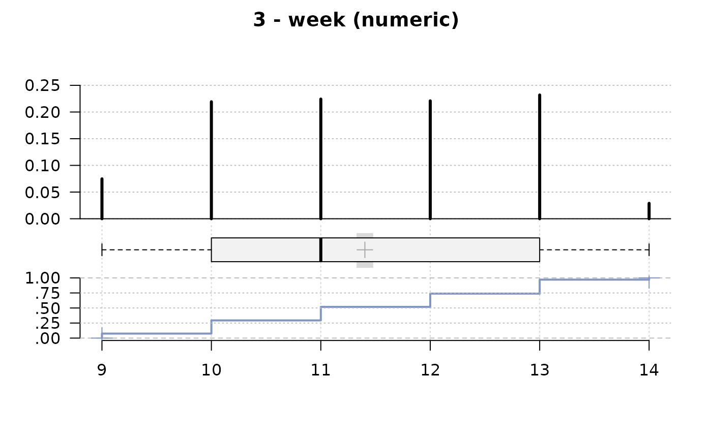
 #> ──────────────────────────────────────────────────────────────────────────────
#> 3 - week (numeric)
#>
#> length n NAs unique 0s mean meanCI'
#> 1'209 1'177 32 6 0 11.40 11.33
#> 97.4% 2.6% 0.0% 11.48
#>
#> .05 .10 .25 median .75 .90 .95
#> 9.00 10.00 10.00 11.00 13.00 13.00 13.00
#>
#> range sd vcoef mad IQR skew kurt
#> 5.00 1.33 0.12 1.48 3.00 -0.07 -1.01
#>
#>
#> value freq perc cumfreq cumperc
#> 1 9 88 7.5% 88 7.5%
#> 2 10 258 21.9% 346 29.4%
#> 3 11 264 22.4% 610 51.8%
#> 4 12 260 22.1% 870 73.9%
#> 5 13 273 23.2% 1'143 97.1%
#> 6 14 34 2.9% 1'177 100.0%
#>
#> ' 95%-CI (classic)
#>
#> ──────────────────────────────────────────────────────────────────────────────
#> 3 - week (numeric)
#>
#> length n NAs unique 0s mean meanCI'
#> 1'209 1'177 32 6 0 11.40 11.33
#> 97.4% 2.6% 0.0% 11.48
#>
#> .05 .10 .25 median .75 .90 .95
#> 9.00 10.00 10.00 11.00 13.00 13.00 13.00
#>
#> range sd vcoef mad IQR skew kurt
#> 5.00 1.33 0.12 1.48 3.00 -0.07 -1.01
#>
#>
#> value freq perc cumfreq cumperc
#> 1 9 88 7.5% 88 7.5%
#> 2 10 258 21.9% 346 29.4%
#> 3 11 264 22.4% 610 51.8%
#> 4 12 260 22.1% 870 73.9%
#> 5 13 273 23.2% 1'143 97.1%
#> 6 14 34 2.9% 1'177 100.0%
#>
#> ' 95%-CI (classic)
#>
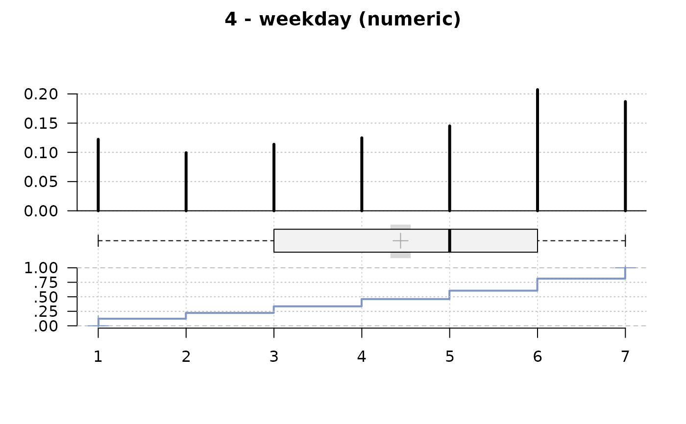
 #> ──────────────────────────────────────────────────────────────────────────────
#> 4 - weekday (numeric)
#>
#> length n NAs unique 0s mean meanCI'
#> 1'209 1'177 32 7 0 4.44 4.33
#> 97.4% 2.6% 0.0% 4.56
#>
#> .05 .10 .25 median .75 .90 .95
#> 1.00 1.00 3.00 5.00 6.00 7.00 7.00
#>
#> range sd vcoef mad IQR skew kurt
#> 6.00 2.02 0.45 2.97 3.00 -0.34 -1.17
#>
#>
#> value freq perc cumfreq cumperc
#> 1 1 144 12.2% 144 12.2%
#> 2 2 117 9.9% 261 22.2%
#> 3 3 134 11.4% 395 33.6%
#> 4 4 147 12.5% 542 46.0%
#> 5 5 171 14.5% 713 60.6%
#> 6 6 244 20.7% 957 81.3%
#> 7 7 220 18.7% 1'177 100.0%
#>
#> ' 95%-CI (classic)
#>
#> ──────────────────────────────────────────────────────────────────────────────
#> 4 - weekday (numeric)
#>
#> length n NAs unique 0s mean meanCI'
#> 1'209 1'177 32 7 0 4.44 4.33
#> 97.4% 2.6% 0.0% 4.56
#>
#> .05 .10 .25 median .75 .90 .95
#> 1.00 1.00 3.00 5.00 6.00 7.00 7.00
#>
#> range sd vcoef mad IQR skew kurt
#> 6.00 2.02 0.45 2.97 3.00 -0.34 -1.17
#>
#>
#> value freq perc cumfreq cumperc
#> 1 1 144 12.2% 144 12.2%
#> 2 2 117 9.9% 261 22.2%
#> 3 3 134 11.4% 395 33.6%
#> 4 4 147 12.5% 542 46.0%
#> 5 5 171 14.5% 713 60.6%
#> 6 6 244 20.7% 957 81.3%
#> 7 7 220 18.7% 1'177 100.0%
#>
#> ' 95%-CI (classic)
#>
 #> ──────────────────────────────────────────────────────────────────────────────
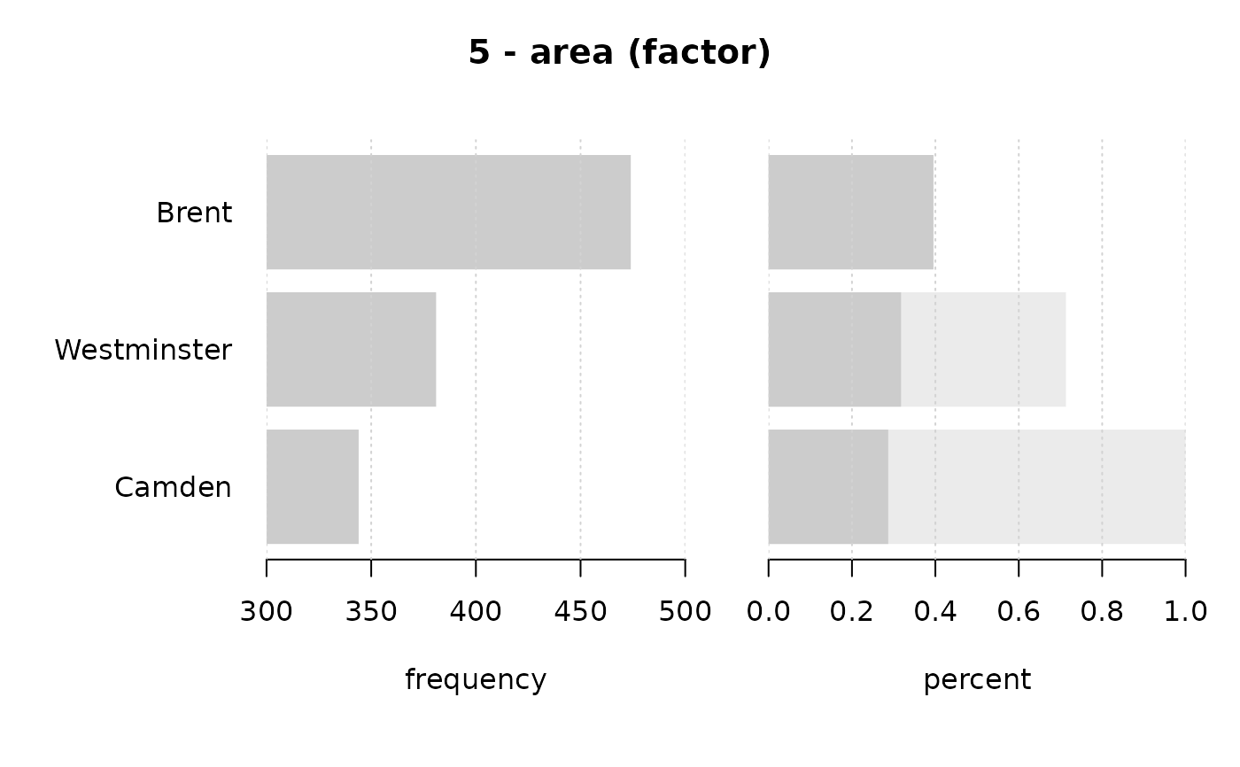
#> 5 - area (factor)
#>
#> length n NAs unique levels dupes
#> 1'209 1'199 10 3 3 y
#> 99.2% 0.8%
#>
#> level freq perc cumfreq cumperc
#> 1 Brent 474 39.5% 474 39.5%
#> 2 Westminster 381 31.8% 855 71.3%
#> 3 Camden 344 28.7% 1'199 100.0%
#>
#> ──────────────────────────────────────────────────────────────────────────────
#> 5 - area (factor)
#>
#> length n NAs unique levels dupes
#> 1'209 1'199 10 3 3 y
#> 99.2% 0.8%
#>
#> level freq perc cumfreq cumperc
#> 1 Brent 474 39.5% 474 39.5%
#> 2 Westminster 381 31.8% 855 71.3%
#> 3 Camden 344 28.7% 1'199 100.0%
#>
 #> ──────────────────────────────────────────────────────────────────────────────
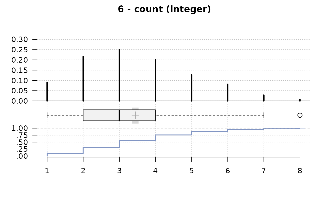
#> 6 - count (integer)
#>
#> length n NAs unique 0s mean meanCI'
#> 1'209 1'197 12 8 0 3.44 3.36
#> 99.0% 1.0% 0.0% 3.53
#>
#> .05 .10 .25 median .75 .90 .95
#> 1.00 2.00 2.00 3.00 4.00 6.00 6.00
#>
#> range sd vcoef mad IQR skew kurt
#> 7.00 1.56 0.45 1.48 2.00 0.45 -0.36
#>
#>
#> value freq perc cumfreq cumperc
#> 1 1 108 9.0% 108 9.0%
#> 2 2 259 21.6% 367 30.7%
#> 3 3 300 25.1% 667 55.7%
#> 4 4 240 20.1% 907 75.8%
#> 5 5 152 12.7% 1'059 88.5%
#> 6 6 97 8.1% 1'156 96.6%
#> 7 7 34 2.8% 1'190 99.4%
#> 8 8 7 0.6% 1'197 100.0%
#>
#> ' 95%-CI (classic)
#>
#> ──────────────────────────────────────────────────────────────────────────────
#> 6 - count (integer)
#>
#> length n NAs unique 0s mean meanCI'
#> 1'209 1'197 12 8 0 3.44 3.36
#> 99.0% 1.0% 0.0% 3.53
#>
#> .05 .10 .25 median .75 .90 .95
#> 1.00 2.00 2.00 3.00 4.00 6.00 6.00
#>
#> range sd vcoef mad IQR skew kurt
#> 7.00 1.56 0.45 1.48 2.00 0.45 -0.36
#>
#>
#> value freq perc cumfreq cumperc
#> 1 1 108 9.0% 108 9.0%
#> 2 2 259 21.6% 367 30.7%
#> 3 3 300 25.1% 667 55.7%
#> 4 4 240 20.1% 907 75.8%
#> 5 5 152 12.7% 1'059 88.5%
#> 6 6 97 8.1% 1'156 96.6%
#> 7 7 34 2.8% 1'190 99.4%
#> 8 8 7 0.6% 1'197 100.0%
#>
#> ' 95%-CI (classic)
#>
 #> ──────────────────────────────────────────────────────────────────────────────
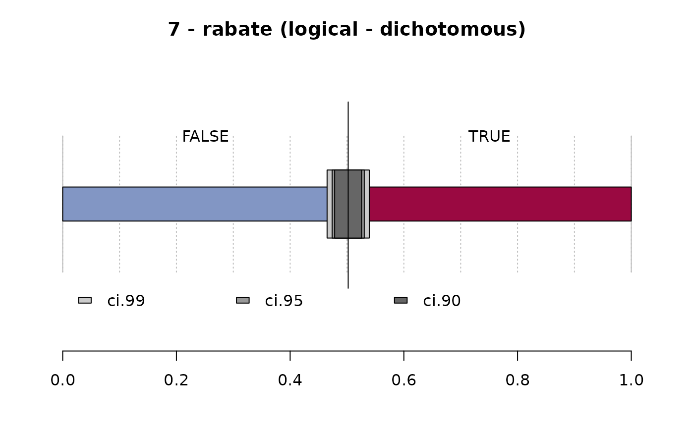
#> 7 - rabate (logical - dichotomous)
#>
#> length n NAs unique
#> 1'209 1'197 12 2
#> 99.0% 1.0%
#>
#> freq perc lci.95 uci.95'
#> FALSE 601 50.2% 47.4% 53.0%
#> TRUE 596 49.8% 47.0% 52.6%
#>
#> ' 95%-CI (Wilson)
#>
#> ──────────────────────────────────────────────────────────────────────────────
#> 7 - rabate (logical - dichotomous)
#>
#> length n NAs unique
#> 1'209 1'197 12 2
#> 99.0% 1.0%
#>
#> freq perc lci.95 uci.95'
#> FALSE 601 50.2% 47.4% 53.0%
#> TRUE 596 49.8% 47.0% 52.6%
#>
#> ' 95%-CI (Wilson)
#>
 #> ──────────────────────────────────────────────────────────────────────────────
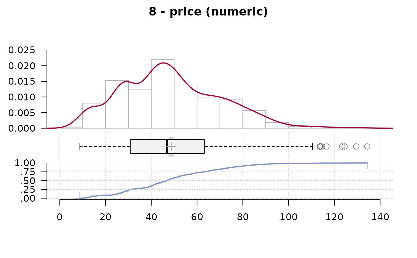
#> 8 - price (numeric)
#>
#> length n NAs unique 0s mean meanCI'
#> 1'209 1'197 12 360 0 48.7289 47.5022
#> 99.0% 1.0% 0.0% 49.9556
#>
#> .05 .10 .25 median .75 .90 .95
#> 13.9900 23.9800 30.9800 46.7640 63.1800 78.8328 87.1200
#>
#> range sd vcoef mad IQR skew kurt
#> 125.5420 21.6313 0.4439 23.4014 32.2000 0.4971 0.1076
#>
#> lowest : 8.792 (3), 9.592, 10.392 (2), 10.99 (11), 11.192 (2)
#> highest: 116.532, 123.39, 124.434, 129.546, 134.334
#>
#> ' 95%-CI (classic)
#>
#> ──────────────────────────────────────────────────────────────────────────────
#> 8 - price (numeric)
#>
#> length n NAs unique 0s mean meanCI'
#> 1'209 1'197 12 360 0 48.7289 47.5022
#> 99.0% 1.0% 0.0% 49.9556
#>
#> .05 .10 .25 median .75 .90 .95
#> 13.9900 23.9800 30.9800 46.7640 63.1800 78.8328 87.1200
#>
#> range sd vcoef mad IQR skew kurt
#> 125.5420 21.6313 0.4439 23.4014 32.2000 0.4971 0.1076
#>
#> lowest : 8.792 (3), 9.592, 10.392 (2), 10.99 (11), 11.192 (2)
#> highest: 116.532, 123.39, 124.434, 129.546, 134.334
#>
#> ' 95%-CI (classic)
#>
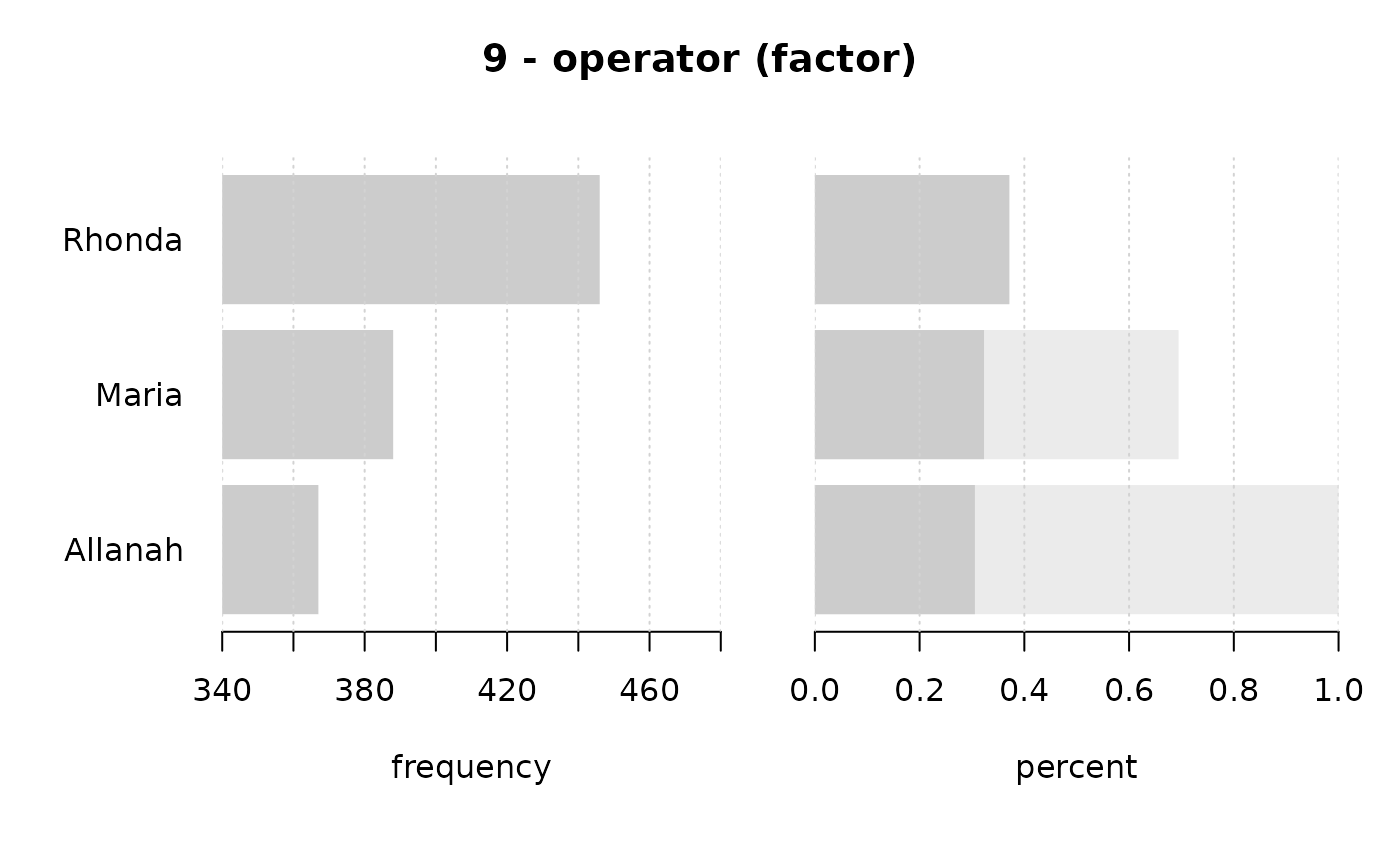
 #> ──────────────────────────────────────────────────────────────────────────────
#> 9 - operator (factor)
#>
#> length n NAs unique levels dupes
#> 1'209 1'201 8 3 3 y
#> 99.3% 0.7%
#>
#> level freq perc cumfreq cumperc
#> 1 Rhonda 446 37.1% 446 37.1%
#> 2 Maria 388 32.3% 834 69.4%
#> 3 Allanah 367 30.6% 1'201 100.0%
#>
#> ──────────────────────────────────────────────────────────────────────────────
#> 9 - operator (factor)
#>
#> length n NAs unique levels dupes
#> 1'209 1'201 8 3 3 y
#> 99.3% 0.7%
#>
#> level freq perc cumfreq cumperc
#> 1 Rhonda 446 37.1% 446 37.1%
#> 2 Maria 388 32.3% 834 69.4%
#> 3 Allanah 367 30.6% 1'201 100.0%
#>
 #> ──────────────────────────────────────────────────────────────────────────────
#> 10 - driver (factor)
#>
#> length n NAs unique levels dupes
#> 1'209 1'204 5 7 7 y
#> 99.6% 0.4%
#>
#> level freq perc cumfreq cumperc
#> 1 Carpenter 272 22.6% 272 22.6%
#> 2 Carter 234 19.4% 506 42.0%
#> 3 Taylor 204 16.9% 710 59.0%
#> 4 Hunter 156 13.0% 866 71.9%
#> 5 Miller 125 10.4% 991 82.3%
#> 6 Farmer 117 9.7% 1'108 92.0%
#> 7 Butcher 96 8.0% 1'204 100.0%
#>
#> ──────────────────────────────────────────────────────────────────────────────
#> 10 - driver (factor)
#>
#> length n NAs unique levels dupes
#> 1'209 1'204 5 7 7 y
#> 99.6% 0.4%
#>
#> level freq perc cumfreq cumperc
#> 1 Carpenter 272 22.6% 272 22.6%
#> 2 Carter 234 19.4% 506 42.0%
#> 3 Taylor 204 16.9% 710 59.0%
#> 4 Hunter 156 13.0% 866 71.9%
#> 5 Miller 125 10.4% 991 82.3%
#> 6 Farmer 117 9.7% 1'108 92.0%
#> 7 Butcher 96 8.0% 1'204 100.0%
#>
 #> ──────────────────────────────────────────────────────────────────────────────
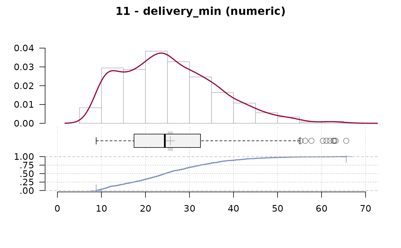
#> 11 - delivery_min (numeric)
#>
#> length n NAs unique 0s mean meanCI'
#> 1'209 1'209 0 384 0 25.65 25.04
#> 100.0% 0.0% 0.0% 26.26
#>
#> .05 .10 .25 median .75 .90 .95
#> 10.40 11.60 17.40 24.40 32.50 40.42 45.20
#>
#> range sd vcoef mad IQR skew kurt
#> 56.80 10.84 0.42 11.27 15.10 0.61 0.10
#>
#> lowest : 8.8 (3), 8.9, 9.0 (3), 9.1 (5), 9.2 (3)
#> highest: 61.9, 62.7, 62.9, 63.2, 65.6
#>
#> ' 95%-CI (classic)
#>
#> ──────────────────────────────────────────────────────────────────────────────
#> 11 - delivery_min (numeric)
#>
#> length n NAs unique 0s mean meanCI'
#> 1'209 1'209 0 384 0 25.65 25.04
#> 100.0% 0.0% 0.0% 26.26
#>
#> .05 .10 .25 median .75 .90 .95
#> 10.40 11.60 17.40 24.40 32.50 40.42 45.20
#>
#> range sd vcoef mad IQR skew kurt
#> 56.80 10.84 0.42 11.27 15.10 0.61 0.10
#>
#> lowest : 8.8 (3), 8.9, 9.0 (3), 9.1 (5), 9.2 (3)
#> highest: 61.9, 62.7, 62.9, 63.2, 65.6
#>
#> ' 95%-CI (classic)
#>
 #> ──────────────────────────────────────────────────────────────────────────────
#> 12 - temperature (numeric)
#>
#> length n NAs unique 0s mean meanCI'
#> 1'209 1'170 39 375 0 47.937 47.367
#> 96.8% 3.2% 0.0% 48.507
#>
#> .05 .10 .25 median .75 .90 .95
#> 26.700 33.290 42.225 50.000 55.300 58.800 60.500
#>
#> range sd vcoef mad IQR skew kurt
#> 45.500 9.938 0.207 9.192 13.075 -0.842 0.051
#>
#> lowest : 19.3, 19.4, 20.0, 20.2 (2), 20.35
#> highest: 63.8, 64.1, 64.6, 64.7, 64.8
#>
#> ' 95%-CI (classic)
#>
#> ──────────────────────────────────────────────────────────────────────────────
#> 12 - temperature (numeric)
#>
#> length n NAs unique 0s mean meanCI'
#> 1'209 1'170 39 375 0 47.937 47.367
#> 96.8% 3.2% 0.0% 48.507
#>
#> .05 .10 .25 median .75 .90 .95
#> 26.700 33.290 42.225 50.000 55.300 58.800 60.500
#>
#> range sd vcoef mad IQR skew kurt
#> 45.500 9.938 0.207 9.192 13.075 -0.842 0.051
#>
#> lowest : 19.3, 19.4, 20.0, 20.2 (2), 20.35
#> highest: 63.8, 64.1, 64.6, 64.7, 64.8
#>
#> ' 95%-CI (classic)
#>
 #> ──────────────────────────────────────────────────────────────────────────────
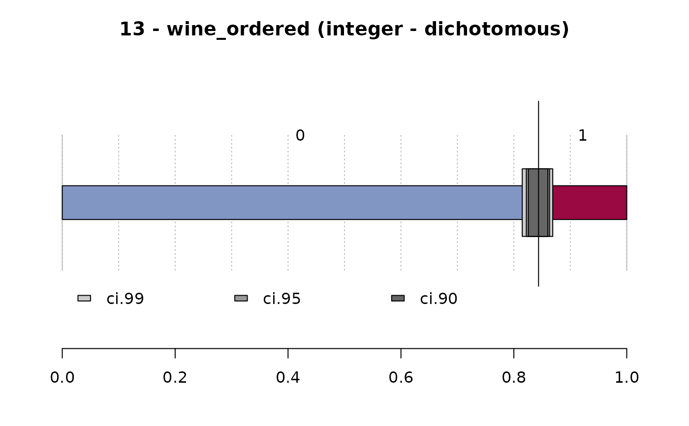
#> 13 - wine_ordered (integer - dichotomous)
#>
#> length n NAs unique
#> 1'209 1'197 12 2
#> 99.0% 1.0%
#>
#> freq perc lci.95 uci.95'
#> 0 1'010 84.4% 82.2% 86.3%
#> 1 187 15.6% 13.7% 17.8%
#>
#> ' 95%-CI (Wilson)
#>
#> ──────────────────────────────────────────────────────────────────────────────
#> 13 - wine_ordered (integer - dichotomous)
#>
#> length n NAs unique
#> 1'209 1'197 12 2
#> 99.0% 1.0%
#>
#> freq perc lci.95 uci.95'
#> 0 1'010 84.4% 82.2% 86.3%
#> 1 187 15.6% 13.7% 17.8%
#>
#> ' 95%-CI (Wilson)
#>
 #> ──────────────────────────────────────────────────────────────────────────────
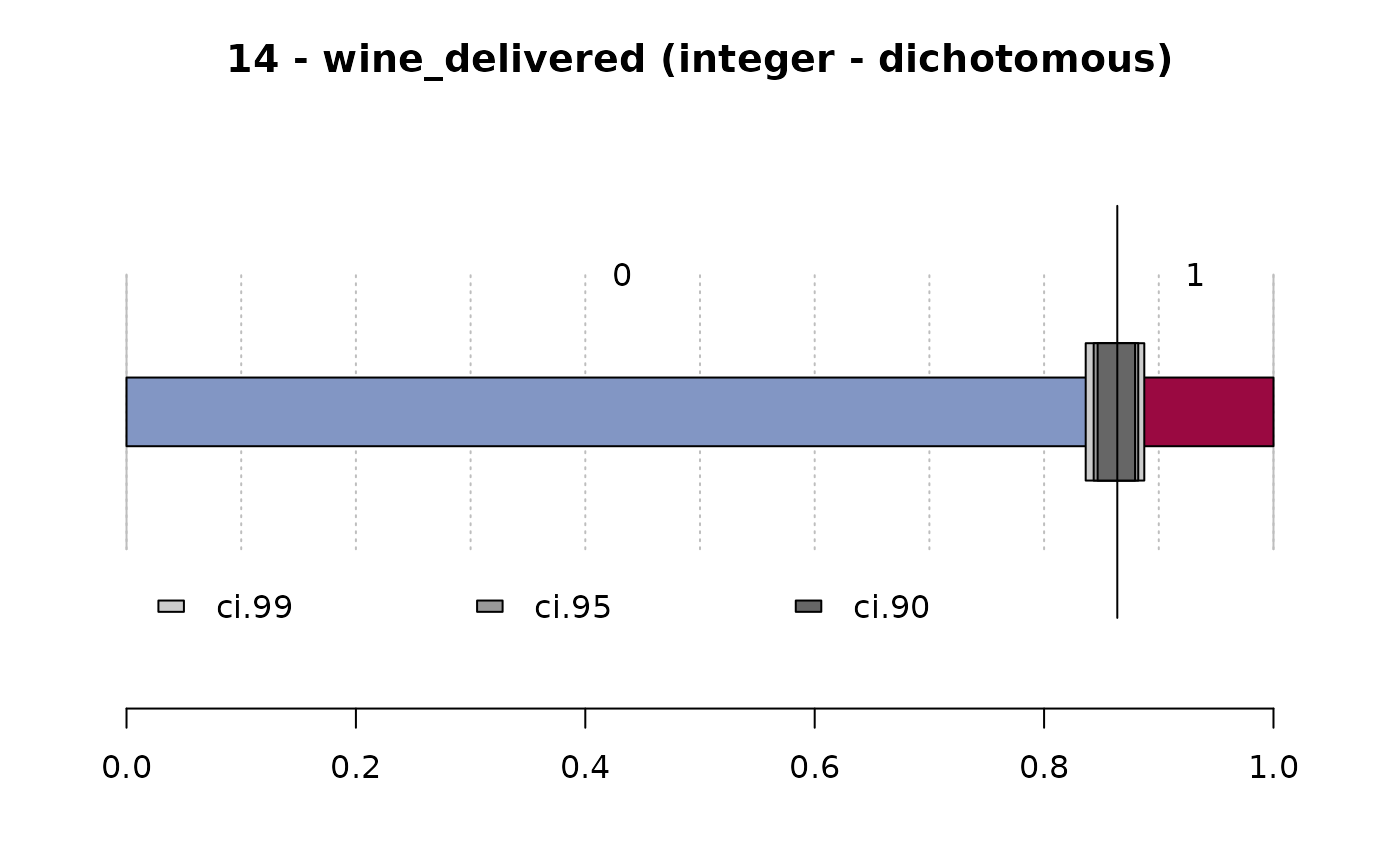
#> 14 - wine_delivered (integer - dichotomous)
#>
#> length n NAs unique
#> 1'209 1'197 12 2
#> 99.0% 1.0%
#>
#> freq perc lci.95 uci.95'
#> 0 1'034 86.4% 84.3% 88.2%
#> 1 163 13.6% 11.8% 15.7%
#>
#> ' 95%-CI (Wilson)
#>
#> ──────────────────────────────────────────────────────────────────────────────
#> 14 - wine_delivered (integer - dichotomous)
#>
#> length n NAs unique
#> 1'209 1'197 12 2
#> 99.0% 1.0%
#>
#> freq perc lci.95 uci.95'
#> 0 1'034 86.4% 84.3% 88.2%
#> 1 163 13.6% 11.8% 15.7%
#>
#> ' 95%-CI (Wilson)
#>
 #> ──────────────────────────────────────────────────────────────────────────────
#> 15 - wrongpizza (logical - dichotomous)
#>
#> length n NAs unique
#> 1'209 1'205 4 2
#> 99.7% 0.3%
#>
#> freq perc lci.95 uci.95'
#> FALSE 1'122 93.1% 91.5% 94.4%
#> TRUE 83 6.9% 5.6% 8.5%
#>
#> ' 95%-CI (Wilson)
#>
#> ──────────────────────────────────────────────────────────────────────────────
#> 15 - wrongpizza (logical - dichotomous)
#>
#> length n NAs unique
#> 1'209 1'205 4 2
#> 99.7% 0.3%
#>
#> freq perc lci.95 uci.95'
#> FALSE 1'122 93.1% 91.5% 94.4%
#> TRUE 83 6.9% 5.6% 8.5%
#>
#> ' 95%-CI (Wilson)
#>
 #> ──────────────────────────────────────────────────────────────────────────────
#> 16 - quality (ordered, factor)
#>
#> length n NAs unique levels dupes
#> 1'209 1'008 201 3 3 y
#> 83.4% 16.6%
#>
#> level freq perc cumfreq cumperc
#> 1 low 156 15.5% 156 15.5%
#> 2 medium 356 35.3% 512 50.8%
#> 3 high 496 49.2% 1'008 100.0%
#>
#> ──────────────────────────────────────────────────────────────────────────────
#> 16 - quality (ordered, factor)
#>
#> length n NAs unique levels dupes
#> 1'209 1'008 201 3 3 y
#> 83.4% 16.6%
#>
#> level freq perc cumfreq cumperc
#> 1 low 156 15.5% 156 15.5%
#> 2 medium 356 35.3% 512 50.8%
#> 3 high 496 49.2% 1'008 100.0%
#>
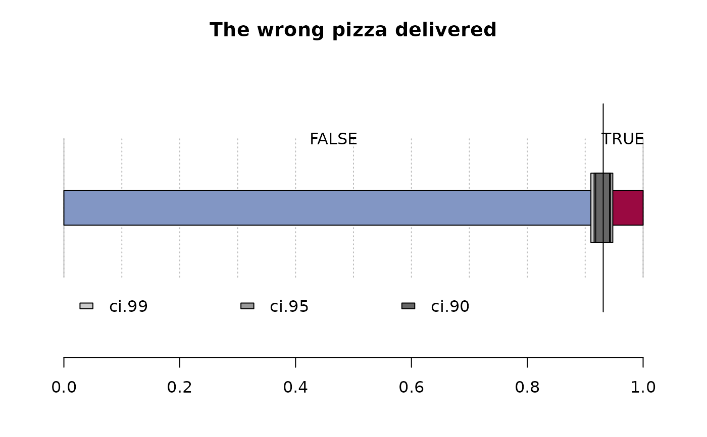
 Desc(d.pizza$wrongpizza, main="The wrong pizza delivered", digits=5)
#> ──────────────────────────────────────────────────────────────────────────────
#> The wrong pizza delivered
#>
#> length n NAs unique
#> 1'209 1'205 4 2
#> 99.7% 0.3%
#>
#> freq perc lci.95 uci.95'
#> FALSE 1'122 93.11203% 91.54086% 94.40921%
#> TRUE 83 6.88797% 5.59079% 8.45914%
#>
#> ' 95%-CI (Wilson)
#>
Desc(d.pizza$wrongpizza, main="The wrong pizza delivered", digits=5)
#> ──────────────────────────────────────────────────────────────────────────────
#> The wrong pizza delivered
#>
#> length n NAs unique
#> 1'209 1'205 4 2
#> 99.7% 0.3%
#>
#> freq perc lci.95 uci.95'
#> FALSE 1'122 93.11203% 91.54086% 94.40921%
#> TRUE 83 6.88797% 5.59079% 8.45914%
#>
#> ' 95%-CI (Wilson)
#>
 Desc(table(d.pizza$area)) # 1-dim table
#> ──────────────────────────────────────────────────────────────────────────────
#> table(d.pizza$area) (table)
#>
#> Summary:
#> n: 1'199, rows: 3
#>
#> Pearson's Chi-squared test (1-dim uniform):
#> X-squared = 22.45, df = 2, p-value = 0.00001333
#>
#> level freq perc cumfreq cumperc
#> 1 Brent 474 39.5% 474 39.5%
#> 2 Camden 344 28.7% 818 68.2%
#> 3 Westminster 381 31.8% 1'199 100.0%
#>
Desc(table(d.pizza$area)) # 1-dim table
#> ──────────────────────────────────────────────────────────────────────────────
#> table(d.pizza$area) (table)
#>
#> Summary:
#> n: 1'199, rows: 3
#>
#> Pearson's Chi-squared test (1-dim uniform):
#> X-squared = 22.45, df = 2, p-value = 0.00001333
#>
#> level freq perc cumfreq cumperc
#> 1 Brent 474 39.5% 474 39.5%
#> 2 Camden 344 28.7% 818 68.2%
#> 3 Westminster 381 31.8% 1'199 100.0%
#>
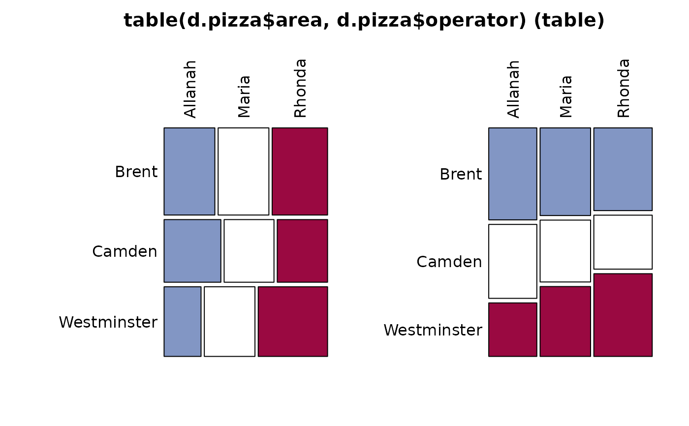
 Desc(table(d.pizza$area, d.pizza$operator)) # 2-dim table
#> ──────────────────────────────────────────────────────────────────────────────
#> table(d.pizza$area, d.pizza$operator) (table)
#>
#> Summary:
#> n: 1'191, rows: 3, columns: 3
#>
#> Pearson's Chi-squared test:
#> X-squared = 17.905, df = 4, p-value = 0.001288
#> Log likelihood ratio (G-test) test of independence:
#> G = 18.099, X-squared df = 4, p-value = 0.001181
#> Mantel-Haenszel Chi-squared:
#> X-squared = 8.6654, df = 1, p-value = 0.003243
#>
#> Contingency Coeff. 0.122
#> Cramer's V 0.087
#> Kendall Tau-b 0.073
#>
#>
#> Allanah Maria Rhonda Sum
#>
#> Brent freq 153 153 167 473
#> perc 12.8% 12.8% 14.0% 39.7%
#> p.row 32.3% 32.3% 35.3% .
#> p.col 41.9% 39.9% 37.7% .
#>
#> Camden freq 123 108 109 340
#> perc 10.3% 9.1% 9.2% 28.5%
#> p.row 36.2% 31.8% 32.1% .
#> p.col 33.7% 28.2% 24.6% .
#>
#> Westminster freq 89 122 167 378
#> perc 7.5% 10.2% 14.0% 31.7%
#> p.row 23.5% 32.3% 44.2% .
#> p.col 24.4% 31.9% 37.7% .
#>
#> Sum freq 365 383 443 1'191
#> perc 30.6% 32.2% 37.2% 100.0%
#> p.row . . . .
#> p.col . . . .
#>
#>
Desc(table(d.pizza$area, d.pizza$operator)) # 2-dim table
#> ──────────────────────────────────────────────────────────────────────────────
#> table(d.pizza$area, d.pizza$operator) (table)
#>
#> Summary:
#> n: 1'191, rows: 3, columns: 3
#>
#> Pearson's Chi-squared test:
#> X-squared = 17.905, df = 4, p-value = 0.001288
#> Log likelihood ratio (G-test) test of independence:
#> G = 18.099, X-squared df = 4, p-value = 0.001181
#> Mantel-Haenszel Chi-squared:
#> X-squared = 8.6654, df = 1, p-value = 0.003243
#>
#> Contingency Coeff. 0.122
#> Cramer's V 0.087
#> Kendall Tau-b 0.073
#>
#>
#> Allanah Maria Rhonda Sum
#>
#> Brent freq 153 153 167 473
#> perc 12.8% 12.8% 14.0% 39.7%
#> p.row 32.3% 32.3% 35.3% .
#> p.col 41.9% 39.9% 37.7% .
#>
#> Camden freq 123 108 109 340
#> perc 10.3% 9.1% 9.2% 28.5%
#> p.row 36.2% 31.8% 32.1% .
#> p.col 33.7% 28.2% 24.6% .
#>
#> Westminster freq 89 122 167 378
#> perc 7.5% 10.2% 14.0% 31.7%
#> p.row 23.5% 32.3% 44.2% .
#> p.col 24.4% 31.9% 37.7% .
#>
#> Sum freq 365 383 443 1'191
#> perc 30.6% 32.2% 37.2% 100.0%
#> p.row . . . .
#> p.col . . . .
#>
#>
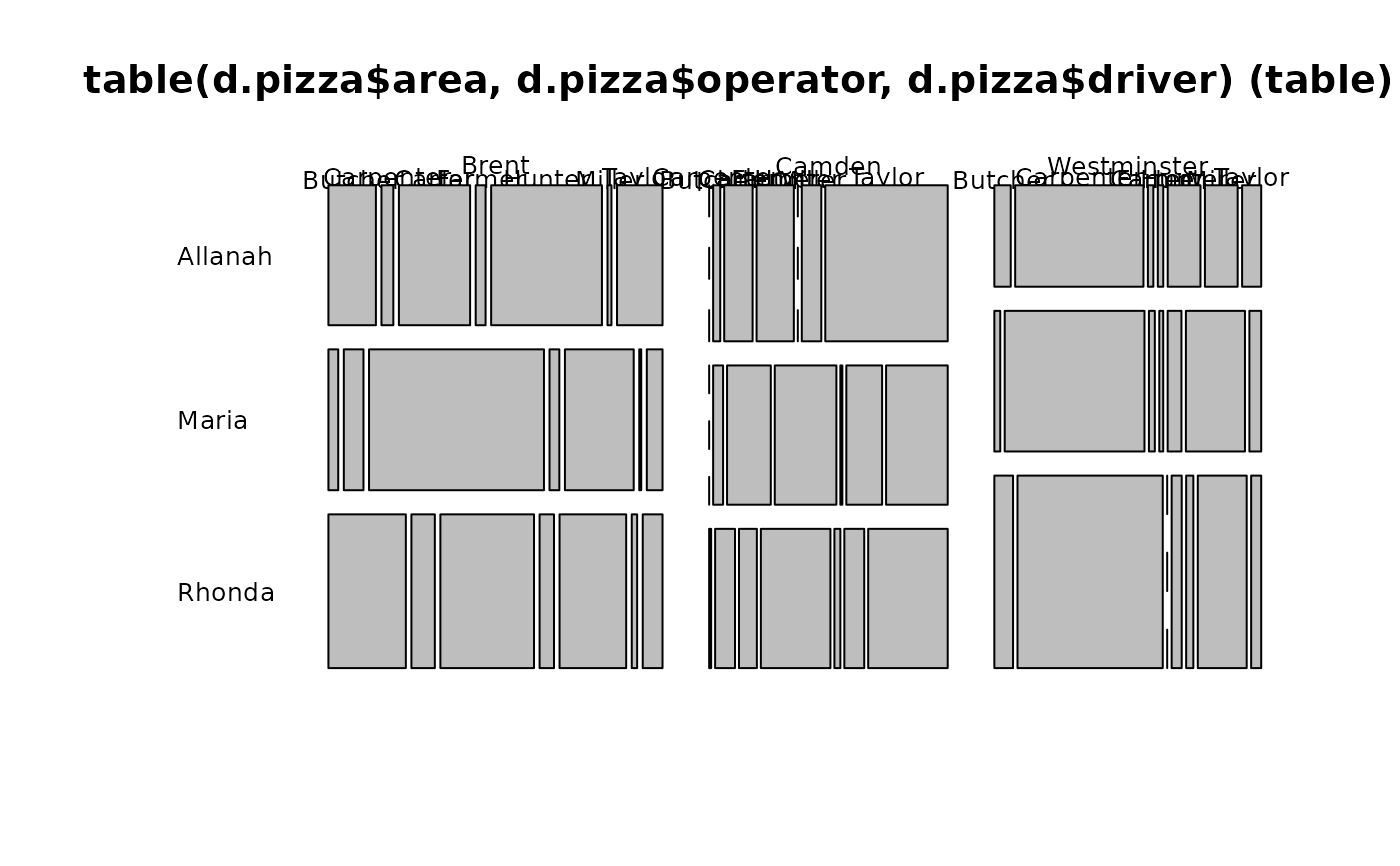
 Desc(table(d.pizza$area, d.pizza$operator, d.pizza$driver)) # n-dim table
#> ──────────────────────────────────────────────────────────────────────────────
#> table(d.pizza$area, d.pizza$operator, d.pizza$driver) (table)
#>
#> Summary:
#> n: 1'186, 3-dim table: 3 x 3 x 7
#>
#> Chi-squared test for independence of all factors:
#> X-squared = 1252.621, df = 52, p-value = < 2.2e-16
#>
#> Butcher Carpenter Carter Farmer Hunter Miller Taylor Sum
#>
#> Brent Allanah 24 6 36 5 56 2 23 152
#> Maria 5 10 89 5 35 1 8 153
#> Rhonda 43 13 52 8 37 3 11 167
#> Camden Allanah 0 4 16 21 0 11 69 121
#> Maria 0 5 22 31 1 18 31 108
#> Rhonda 1 10 9 35 3 10 40 108
#> Westminster Allanah 6 47 2 2 12 12 7 88
#> Maria 3 71 3 2 7 30 6 122
#> Rhonda 13 101 0 7 5 34 7 167
#> Sum Allanah 30 57 54 28 68 25 99 361
#> Maria 8 86 114 38 43 49 45 383
#> Rhonda 57 124 61 50 45 47 58 442
#>
Desc(table(d.pizza$area, d.pizza$operator, d.pizza$driver)) # n-dim table
#> ──────────────────────────────────────────────────────────────────────────────
#> table(d.pizza$area, d.pizza$operator, d.pizza$driver) (table)
#>
#> Summary:
#> n: 1'186, 3-dim table: 3 x 3 x 7
#>
#> Chi-squared test for independence of all factors:
#> X-squared = 1252.621, df = 52, p-value = < 2.2e-16
#>
#> Butcher Carpenter Carter Farmer Hunter Miller Taylor Sum
#>
#> Brent Allanah 24 6 36 5 56 2 23 152
#> Maria 5 10 89 5 35 1 8 153
#> Rhonda 43 13 52 8 37 3 11 167
#> Camden Allanah 0 4 16 21 0 11 69 121
#> Maria 0 5 22 31 1 18 31 108
#> Rhonda 1 10 9 35 3 10 40 108
#> Westminster Allanah 6 47 2 2 12 12 7 88
#> Maria 3 71 3 2 7 30 6 122
#> Rhonda 13 101 0 7 5 34 7 167
#> Sum Allanah 30 57 54 28 68 25 99 361
#> Maria 8 86 114 38 43 49 45 383
#> Rhonda 57 124 61 50 45 47 58 442
#>
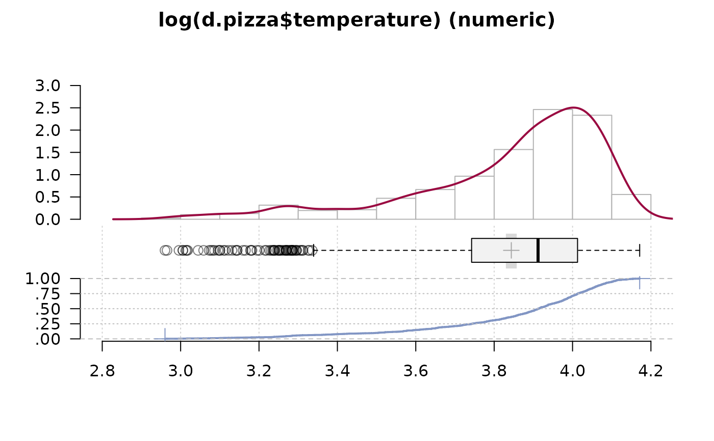
 # expressions
Desc(log(d.pizza$temperature))
#> ──────────────────────────────────────────────────────────────────────────────
#> log(d.pizza$temperature) (numeric)
#>
#> length n NAs unique 0s mean meanCI'
#> 1'209 1'170 39 375 0 3.843745 3.829891
#> 96.8% 3.2% 0.0% 3.857599
#>
#> .05 .10 .25 median .75 .90 .95
#> 3.284664 3.505257 3.743012 3.912023 4.012773 4.074142 4.102643
#>
#> range sd vcoef mad IQR skew kurt
#> 1.211201 0.241536 0.062839 0.181200 0.269761 -1.377446 1.528453
#>
#> lowest : 2.960105, 2.965273, 2.995732, 3.005683 (2), 3.013081
#> highest: 4.155753, 4.160444, 4.168214, 4.169761, 4.171306
#>
#> ' 95%-CI (classic)
#>
# expressions
Desc(log(d.pizza$temperature))
#> ──────────────────────────────────────────────────────────────────────────────
#> log(d.pizza$temperature) (numeric)
#>
#> length n NAs unique 0s mean meanCI'
#> 1'209 1'170 39 375 0 3.843745 3.829891
#> 96.8% 3.2% 0.0% 3.857599
#>
#> .05 .10 .25 median .75 .90 .95
#> 3.284664 3.505257 3.743012 3.912023 4.012773 4.074142 4.102643
#>
#> range sd vcoef mad IQR skew kurt
#> 1.211201 0.241536 0.062839 0.181200 0.269761 -1.377446 1.528453
#>
#> lowest : 2.960105, 2.965273, 2.995732, 3.005683 (2), 3.013081
#> highest: 4.155753, 4.160444, 4.168214, 4.169761, 4.171306
#>
#> ' 95%-CI (classic)
#>
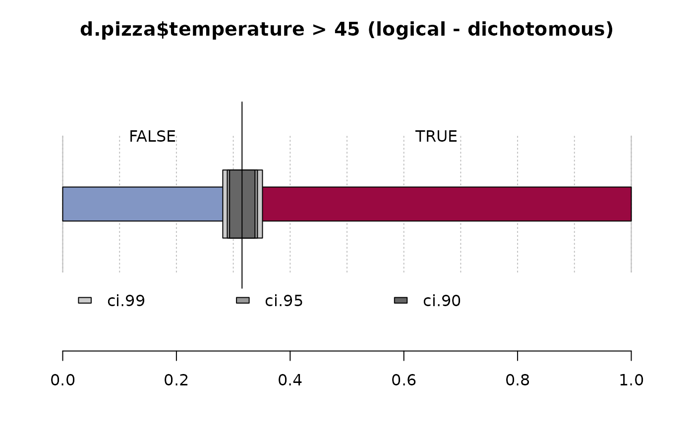
 Desc(d.pizza$temperature > 45)
#> ──────────────────────────────────────────────────────────────────────────────
#> d.pizza$temperature > 45 (logical - dichotomous)
#>
#> length n NAs unique
#> 1'209 1'170 39 2
#> 96.8% 3.2%
#>
#> freq perc lci.95 uci.95'
#> FALSE 369 31.5% 28.9% 34.3%
#> TRUE 801 68.5% 65.7% 71.1%
#>
#> ' 95%-CI (Wilson)
#>
Desc(d.pizza$temperature > 45)
#> ──────────────────────────────────────────────────────────────────────────────
#> d.pizza$temperature > 45 (logical - dichotomous)
#>
#> length n NAs unique
#> 1'209 1'170 39 2
#> 96.8% 3.2%
#>
#> freq perc lci.95 uci.95'
#> FALSE 369 31.5% 28.9% 34.3%
#> TRUE 801 68.5% 65.7% 71.1%
#>
#> ' 95%-CI (Wilson)
#>
 # supported labels
Label(d.pizza$temperature) <- "This is the temperature in degrees Celsius
measured at the time when the pizza is delivered to the client."
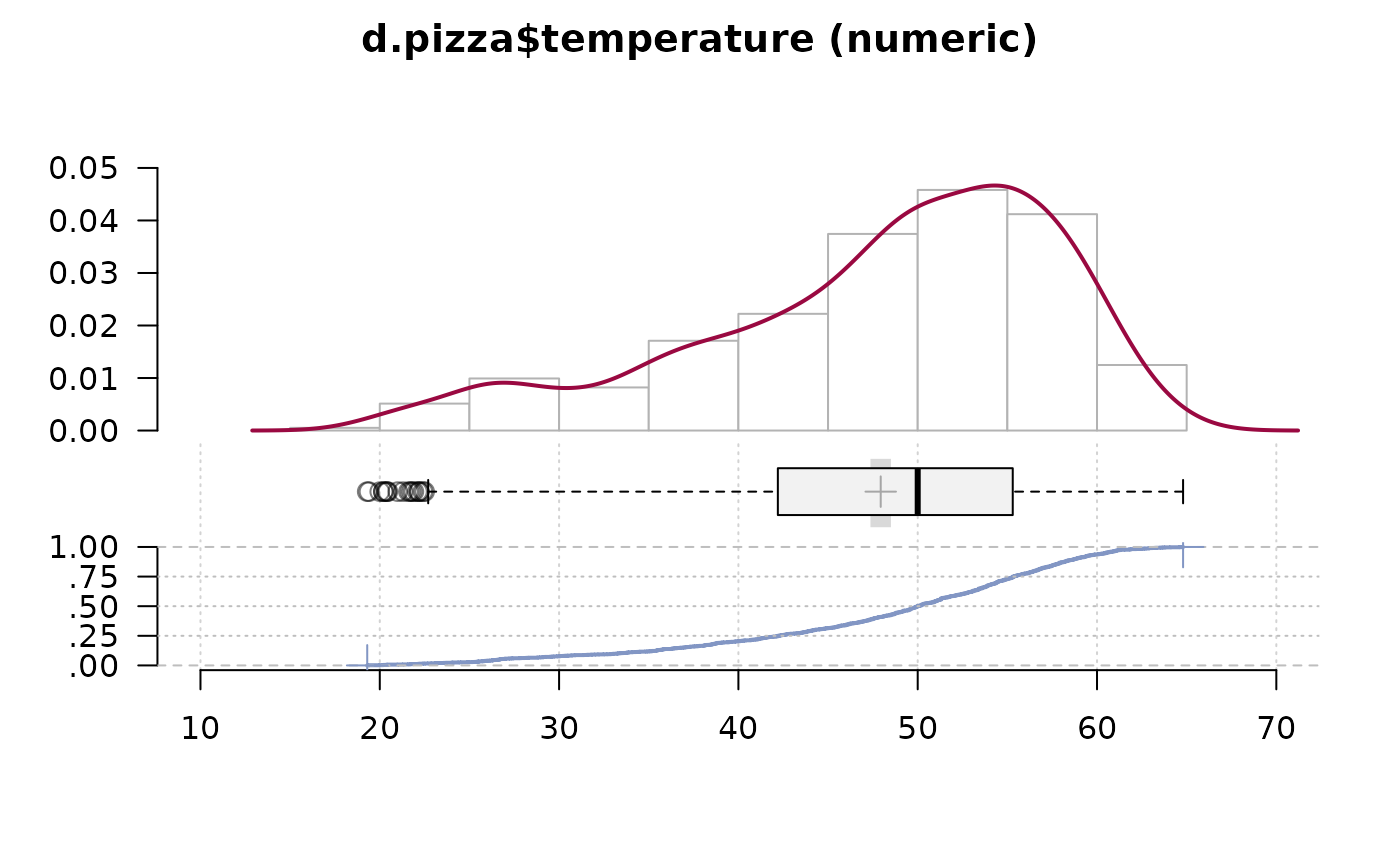
Desc(d.pizza$temperature)
#> ──────────────────────────────────────────────────────────────────────────────
#> d.pizza$temperature (numeric) :
#> This is the temperature in degrees Celsius measured at the time when
#> the pizza is delivered to the client.
#>
#>
#> length n NAs unique 0s mean meanCI'
#> 1'209 1'170 39 375 0 47.937 47.367
#> 96.8% 3.2% 0.0% 48.507
#>
#> .05 .10 .25 median .75 .90 .95
#> 26.700 33.290 42.225 50.000 55.300 58.800 60.500
#>
#> range sd vcoef mad IQR skew kurt
#> 45.500 9.938 0.207 9.192 13.075 -0.842 0.051
#>
#> lowest : 19.3, 19.4, 20.0, 20.2 (2), 20.35
#> highest: 63.8, 64.1, 64.6, 64.7, 64.8
#>
#> ' 95%-CI (classic)
#>
# supported labels
Label(d.pizza$temperature) <- "This is the temperature in degrees Celsius
measured at the time when the pizza is delivered to the client."
Desc(d.pizza$temperature)
#> ──────────────────────────────────────────────────────────────────────────────
#> d.pizza$temperature (numeric) :
#> This is the temperature in degrees Celsius measured at the time when
#> the pizza is delivered to the client.
#>
#>
#> length n NAs unique 0s mean meanCI'
#> 1'209 1'170 39 375 0 47.937 47.367
#> 96.8% 3.2% 0.0% 48.507
#>
#> .05 .10 .25 median .75 .90 .95
#> 26.700 33.290 42.225 50.000 55.300 58.800 60.500
#>
#> range sd vcoef mad IQR skew kurt
#> 45.500 9.938 0.207 9.192 13.075 -0.842 0.051
#>
#> lowest : 19.3, 19.4, 20.0, 20.2 (2), 20.35
#> highest: 63.8, 64.1, 64.6, 64.7, 64.8
#>
#> ' 95%-CI (classic)
#>
 # try as well: Desc(d.pizza$temperature, wrd=GetNewWrd())
z <- Desc(d.pizza$temperature)
print(z, digits=1, plotit=FALSE)
#> ──────────────────────────────────────────────────────────────────────────────
#> d.pizza$temperature (numeric) :
#> This is the temperature in degrees Celsius measured at the time when
#> the pizza is delivered to the client.
#>
#>
#> length n NAs unique 0s mean meanCI'
#> 1'209 1'170 39 375 0 47.9 47.4
#> 96.8% 3.2% 0.0% 48.5
#>
#> .05 .10 .25 median .75 .90 .95
#> 26.7 33.3 42.2 50.0 55.3 58.8 60.5
#>
#> range sd vcoef mad IQR skew kurt
#> 45.5 9.9 0.2 9.2 13.1 -0.8 0.1
#>
#> lowest : 19.3, 19.4, 20.0, 20.2 (2), 20.4
#> highest: 63.8, 64.1, 64.6, 64.7, 64.8
#>
#> ' 95%-CI (classic)
#>
# plot (additional arguments are passed on to the underlying plot function)
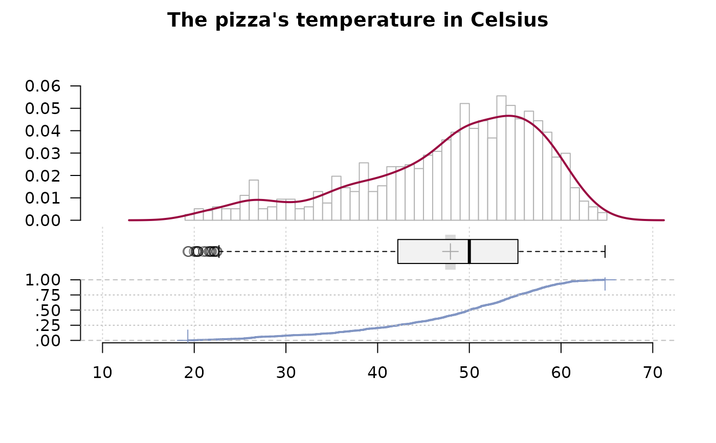
plot(z, main="The pizza's temperature in Celsius", args.hist=list(breaks=50))
# try as well: Desc(d.pizza$temperature, wrd=GetNewWrd())
z <- Desc(d.pizza$temperature)
print(z, digits=1, plotit=FALSE)
#> ──────────────────────────────────────────────────────────────────────────────
#> d.pizza$temperature (numeric) :
#> This is the temperature in degrees Celsius measured at the time when
#> the pizza is delivered to the client.
#>
#>
#> length n NAs unique 0s mean meanCI'
#> 1'209 1'170 39 375 0 47.9 47.4
#> 96.8% 3.2% 0.0% 48.5
#>
#> .05 .10 .25 median .75 .90 .95
#> 26.7 33.3 42.2 50.0 55.3 58.8 60.5
#>
#> range sd vcoef mad IQR skew kurt
#> 45.5 9.9 0.2 9.2 13.1 -0.8 0.1
#>
#> lowest : 19.3, 19.4, 20.0, 20.2 (2), 20.4
#> highest: 63.8, 64.1, 64.6, 64.7, 64.8
#>
#> ' 95%-CI (classic)
#>
# plot (additional arguments are passed on to the underlying plot function)
plot(z, main="The pizza's temperature in Celsius", args.hist=list(breaks=50))
 # formula interface for single variables
Desc(~ uptake + Type, data = CO2, plotit = FALSE)
#> ──────────────────────────────────────────────────────────────────────────────
#> CO2$uptake (numeric)
#>
#> length n NAs unique 0s mean meanCI'
#> 84 84 0 76 0 27.213 24.866
#> 100.0% 0.0% 0.0% 29.560
#>
#> .05 .10 .25 median .75 .90 .95
#> 10.705 12.360 17.900 28.300 37.125 41.160 42.355
#>
#> range sd vcoef mad IQR skew kurt
#> 37.800 10.814 0.397 14.826 19.225 -0.104 -1.348
#>
#> lowest : 7.7, 9.3, 10.5, 10.6 (2), 11.3
#> highest: 42.4, 42.9, 43.9, 44.3, 45.5
#>
#> ' 95%-CI (classic)
#>
#> ──────────────────────────────────────────────────────────────────────────────
#> CO2$Type (logical)
#>
#> length n NAs unique
#> 84 84 0 2
#> 100.0% 0.0%
#>
#> freq perc lci.95 uci.95'
#> Quebec 42 50.0% 39.5% 60.5%
#> Mississippi 42 50.0% 39.5% 60.5%
#>
#> ' 95%-CI (Wilson)
#>
# bivariate
Desc(price ~ operator, data=d.pizza) # numeric ~ factor
#> ──────────────────────────────────────────────────────────────────────────────
#> price ~ operator (d.pizza)
#>
#> Summary:
#> n pairs: 1'209, valid: 1'189 (98.3%), missings: 20 (1.7%), groups: 3
#>
#>
#> Allanah Maria Rhonda
#> mean 46.30693 49.11556 50.37397
#> median 44.97000 46.76400 47.97000
#> sd 20.15232 21.97820 22.41006
#> IQR 28.86780 31.82800 33.43175
#> n 363 384 442
#> np 30.52986% 32.29605% 37.17410%
#> NAs 4 4 4
#> 0s 0 0 0
#>
#> Kruskal-Wallis rank sum test:
#> Kruskal-Wallis chi-squared = 6.2048, df = 2, p-value = 0.04494
#>
#>
#> Warning:
#> Grouping variable contains 8 NAs (0.662%).
#>
# formula interface for single variables
Desc(~ uptake + Type, data = CO2, plotit = FALSE)
#> ──────────────────────────────────────────────────────────────────────────────
#> CO2$uptake (numeric)
#>
#> length n NAs unique 0s mean meanCI'
#> 84 84 0 76 0 27.213 24.866
#> 100.0% 0.0% 0.0% 29.560
#>
#> .05 .10 .25 median .75 .90 .95
#> 10.705 12.360 17.900 28.300 37.125 41.160 42.355
#>
#> range sd vcoef mad IQR skew kurt
#> 37.800 10.814 0.397 14.826 19.225 -0.104 -1.348
#>
#> lowest : 7.7, 9.3, 10.5, 10.6 (2), 11.3
#> highest: 42.4, 42.9, 43.9, 44.3, 45.5
#>
#> ' 95%-CI (classic)
#>
#> ──────────────────────────────────────────────────────────────────────────────
#> CO2$Type (logical)
#>
#> length n NAs unique
#> 84 84 0 2
#> 100.0% 0.0%
#>
#> freq perc lci.95 uci.95'
#> Quebec 42 50.0% 39.5% 60.5%
#> Mississippi 42 50.0% 39.5% 60.5%
#>
#> ' 95%-CI (Wilson)
#>
# bivariate
Desc(price ~ operator, data=d.pizza) # numeric ~ factor
#> ──────────────────────────────────────────────────────────────────────────────
#> price ~ operator (d.pizza)
#>
#> Summary:
#> n pairs: 1'209, valid: 1'189 (98.3%), missings: 20 (1.7%), groups: 3
#>
#>
#> Allanah Maria Rhonda
#> mean 46.30693 49.11556 50.37397
#> median 44.97000 46.76400 47.97000
#> sd 20.15232 21.97820 22.41006
#> IQR 28.86780 31.82800 33.43175
#> n 363 384 442
#> np 30.52986% 32.29605% 37.17410%
#> NAs 4 4 4
#> 0s 0 0 0
#>
#> Kruskal-Wallis rank sum test:
#> Kruskal-Wallis chi-squared = 6.2048, df = 2, p-value = 0.04494
#>
#>
#> Warning:
#> Grouping variable contains 8 NAs (0.662%).
#>
 Desc(driver ~ operator, data=d.pizza) # factor ~ factor
#> ──────────────────────────────────────────────────────────────────────────────
#> driver ~ operator (d.pizza)
#>
#> Summary:
#> n: 1'196, rows: 3, columns: 7
#>
#> Pearson's Chi-squared test:
#> X-squared = 133.06, df = 12, p-value < 2.2e-16
#> Log likelihood ratio (G-test) test of independence:
#> G = 133.53, X-squared df = 12, p-value < 2.2e-16
#> Mantel-Haenszel Chi-squared:
#> X-squared = 33.539, df = 1, p-value = 0.000000006984
#>
#> Contingency Coeff. 0.316
#> Cramer's V 0.236
#> Kendall Tau-b -0.145
#>
#>
#> driver Butcher Carpenter Carter Farmer Hunter Miller
#> operator
#>
#> Allanah freq 30 58 55 28 68 25
#> perc 2.5% 4.8% 4.6% 2.3% 5.7% 2.1%
#> p.row 8.3% 16.0% 15.2% 7.7% 18.7% 6.9%
#> p.col 31.2% 21.5% 23.5% 24.1% 43.6% 20.5%
#>
#> Maria freq 8 87 117 38 43 50
#> perc 0.7% 7.3% 9.8% 3.2% 3.6% 4.2%
#> p.row 2.1% 22.4% 30.2% 9.8% 11.1% 12.9%
#> p.col 8.3% 32.2% 50.0% 32.8% 27.6% 41.0%
#>
#> Rhonda freq 58 125 62 50 45 47
#> perc 4.8% 10.5% 5.2% 4.2% 3.8% 3.9%
#> p.row 13.0% 28.1% 13.9% 11.2% 10.1% 10.6%
#> p.col 60.4% 46.3% 26.5% 43.1% 28.8% 38.5%
#>
#> Sum freq 96 270 234 116 156 122
#> perc 8.0% 22.6% 19.6% 9.7% 13.0% 10.2%
#> p.row . . . . . .
#> p.col . . . . . .
#>
#>
#> driver Taylor Sum
#> operator
#>
#> Allanah freq 99 363
#> perc 8.3% 30.4%
#> p.row 27.3% .
#> p.col 49.0% .
#>
#> Maria freq 45 388
#> perc 3.8% 32.4%
#> p.row 11.6% .
#> p.col 22.3% .
#>
#> Rhonda freq 58 445
#> perc 4.8% 37.2%
#> p.row 13.0% .
#> p.col 28.7% .
#>
#> Sum freq 202 1'196
#> perc 16.9% 100.0%
#> p.row . .
#> p.col . .
#>
#>
Desc(driver ~ operator, data=d.pizza) # factor ~ factor
#> ──────────────────────────────────────────────────────────────────────────────
#> driver ~ operator (d.pizza)
#>
#> Summary:
#> n: 1'196, rows: 3, columns: 7
#>
#> Pearson's Chi-squared test:
#> X-squared = 133.06, df = 12, p-value < 2.2e-16
#> Log likelihood ratio (G-test) test of independence:
#> G = 133.53, X-squared df = 12, p-value < 2.2e-16
#> Mantel-Haenszel Chi-squared:
#> X-squared = 33.539, df = 1, p-value = 0.000000006984
#>
#> Contingency Coeff. 0.316
#> Cramer's V 0.236
#> Kendall Tau-b -0.145
#>
#>
#> driver Butcher Carpenter Carter Farmer Hunter Miller
#> operator
#>
#> Allanah freq 30 58 55 28 68 25
#> perc 2.5% 4.8% 4.6% 2.3% 5.7% 2.1%
#> p.row 8.3% 16.0% 15.2% 7.7% 18.7% 6.9%
#> p.col 31.2% 21.5% 23.5% 24.1% 43.6% 20.5%
#>
#> Maria freq 8 87 117 38 43 50
#> perc 0.7% 7.3% 9.8% 3.2% 3.6% 4.2%
#> p.row 2.1% 22.4% 30.2% 9.8% 11.1% 12.9%
#> p.col 8.3% 32.2% 50.0% 32.8% 27.6% 41.0%
#>
#> Rhonda freq 58 125 62 50 45 47
#> perc 4.8% 10.5% 5.2% 4.2% 3.8% 3.9%
#> p.row 13.0% 28.1% 13.9% 11.2% 10.1% 10.6%
#> p.col 60.4% 46.3% 26.5% 43.1% 28.8% 38.5%
#>
#> Sum freq 96 270 234 116 156 122
#> perc 8.0% 22.6% 19.6% 9.7% 13.0% 10.2%
#> p.row . . . . . .
#> p.col . . . . . .
#>
#>
#> driver Taylor Sum
#> operator
#>
#> Allanah freq 99 363
#> perc 8.3% 30.4%
#> p.row 27.3% .
#> p.col 49.0% .
#>
#> Maria freq 45 388
#> perc 3.8% 32.4%
#> p.row 11.6% .
#> p.col 22.3% .
#>
#> Rhonda freq 58 445
#> perc 4.8% 37.2%
#> p.row 13.0% .
#> p.col 28.7% .
#>
#> Sum freq 202 1'196
#> perc 16.9% 100.0%
#> p.row . .
#> p.col . .
#>
#>
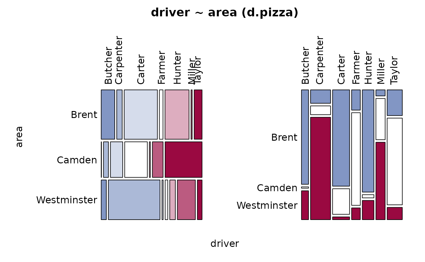
 Desc(driver ~ area + operator, data=d.pizza) # factor ~ several factors
#> ──────────────────────────────────────────────────────────────────────────────
#> driver ~ area (d.pizza)
#>
#> Summary:
#> n: 1'194, rows: 3, columns: 7
#>
#> Pearson's Chi-squared test:
#> X-squared = 1009.5, df = 12, p-value < 2.2e-16
#> Log likelihood ratio (G-test) test of independence:
#> G = 1020.9, X-squared df = 12, p-value < 2.2e-16
#> Mantel-Haenszel Chi-squared:
#> X-squared = 2.6144, df = 1, p-value = 0.1059
#>
#> Contingency Coeff. 0.677
#> Cramer's V 0.650
#> Kendall Tau-b -0.057
#>
#>
#> driver Butcher Carpenter Carter Farmer Hunter Miller
#> area
#>
#> Brent freq 72 29 177 19 128 6
#> perc 6.0% 2.4% 14.8% 1.6% 10.7% 0.5%
#> p.row 15.2% 6.1% 37.4% 4.0% 27.1% 1.3%
#> p.col 75.8% 10.8% 77.3% 16.2% 82.1% 4.8%
#>
#> Camden freq 1 19 47 87 4 41
#> perc 0.1% 1.6% 3.9% 7.3% 0.3% 3.4%
#> p.row 0.3% 5.6% 13.8% 25.5% 1.2% 12.0%
#> p.col 1.1% 7.1% 20.5% 74.4% 2.6% 33.1%
#>
#> Westminster freq 22 221 5 11 24 77
#> perc 1.8% 18.5% 0.4% 0.9% 2.0% 6.4%
#> p.row 5.8% 58.2% 1.3% 2.9% 6.3% 20.3%
#> p.col 23.2% 82.2% 2.2% 9.4% 15.4% 62.1%
#>
#> Sum freq 95 269 229 117 156 124
#> perc 8.0% 22.5% 19.2% 9.8% 13.1% 10.4%
#> p.row . . . . . .
#> p.col . . . . . .
#>
#>
#> driver Taylor Sum
#> area
#>
#> Brent freq 42 473
#> perc 3.5% 39.6%
#> p.row 8.9% .
#> p.col 20.6% .
#>
#> Camden freq 142 341
#> perc 11.9% 28.6%
#> p.row 41.6% .
#> p.col 69.6% .
#>
#> Westminster freq 20 380
#> perc 1.7% 31.8%
#> p.row 5.3% .
#> p.col 9.8% .
#>
#> Sum freq 204 1'194
#> perc 17.1% 100.0%
#> p.row . .
#> p.col . .
#>
#>
Desc(driver ~ area + operator, data=d.pizza) # factor ~ several factors
#> ──────────────────────────────────────────────────────────────────────────────
#> driver ~ area (d.pizza)
#>
#> Summary:
#> n: 1'194, rows: 3, columns: 7
#>
#> Pearson's Chi-squared test:
#> X-squared = 1009.5, df = 12, p-value < 2.2e-16
#> Log likelihood ratio (G-test) test of independence:
#> G = 1020.9, X-squared df = 12, p-value < 2.2e-16
#> Mantel-Haenszel Chi-squared:
#> X-squared = 2.6144, df = 1, p-value = 0.1059
#>
#> Contingency Coeff. 0.677
#> Cramer's V 0.650
#> Kendall Tau-b -0.057
#>
#>
#> driver Butcher Carpenter Carter Farmer Hunter Miller
#> area
#>
#> Brent freq 72 29 177 19 128 6
#> perc 6.0% 2.4% 14.8% 1.6% 10.7% 0.5%
#> p.row 15.2% 6.1% 37.4% 4.0% 27.1% 1.3%
#> p.col 75.8% 10.8% 77.3% 16.2% 82.1% 4.8%
#>
#> Camden freq 1 19 47 87 4 41
#> perc 0.1% 1.6% 3.9% 7.3% 0.3% 3.4%
#> p.row 0.3% 5.6% 13.8% 25.5% 1.2% 12.0%
#> p.col 1.1% 7.1% 20.5% 74.4% 2.6% 33.1%
#>
#> Westminster freq 22 221 5 11 24 77
#> perc 1.8% 18.5% 0.4% 0.9% 2.0% 6.4%
#> p.row 5.8% 58.2% 1.3% 2.9% 6.3% 20.3%
#> p.col 23.2% 82.2% 2.2% 9.4% 15.4% 62.1%
#>
#> Sum freq 95 269 229 117 156 124
#> perc 8.0% 22.5% 19.2% 9.8% 13.1% 10.4%
#> p.row . . . . . .
#> p.col . . . . . .
#>
#>
#> driver Taylor Sum
#> area
#>
#> Brent freq 42 473
#> perc 3.5% 39.6%
#> p.row 8.9% .
#> p.col 20.6% .
#>
#> Camden freq 142 341
#> perc 11.9% 28.6%
#> p.row 41.6% .
#> p.col 69.6% .
#>
#> Westminster freq 20 380
#> perc 1.7% 31.8%
#> p.row 5.3% .
#> p.col 9.8% .
#>
#> Sum freq 204 1'194
#> perc 17.1% 100.0%
#> p.row . .
#> p.col . .
#>
#>
 #> ──────────────────────────────────────────────────────────────────────────────
#> driver ~ operator (d.pizza)
#>
#> Summary:
#> n: 1'196, rows: 3, columns: 7
#>
#> Pearson's Chi-squared test:
#> X-squared = 133.06, df = 12, p-value < 2.2e-16
#> Log likelihood ratio (G-test) test of independence:
#> G = 133.53, X-squared df = 12, p-value < 2.2e-16
#> Mantel-Haenszel Chi-squared:
#> X-squared = 33.539, df = 1, p-value = 0.000000006984
#>
#> Contingency Coeff. 0.316
#> Cramer's V 0.236
#> Kendall Tau-b -0.145
#>
#>
#> driver Butcher Carpenter Carter Farmer Hunter Miller
#> operator
#>
#> Allanah freq 30 58 55 28 68 25
#> perc 2.5% 4.8% 4.6% 2.3% 5.7% 2.1%
#> p.row 8.3% 16.0% 15.2% 7.7% 18.7% 6.9%
#> p.col 31.2% 21.5% 23.5% 24.1% 43.6% 20.5%
#>
#> Maria freq 8 87 117 38 43 50
#> perc 0.7% 7.3% 9.8% 3.2% 3.6% 4.2%
#> p.row 2.1% 22.4% 30.2% 9.8% 11.1% 12.9%
#> p.col 8.3% 32.2% 50.0% 32.8% 27.6% 41.0%
#>
#> Rhonda freq 58 125 62 50 45 47
#> perc 4.8% 10.5% 5.2% 4.2% 3.8% 3.9%
#> p.row 13.0% 28.1% 13.9% 11.2% 10.1% 10.6%
#> p.col 60.4% 46.3% 26.5% 43.1% 28.8% 38.5%
#>
#> Sum freq 96 270 234 116 156 122
#> perc 8.0% 22.6% 19.6% 9.7% 13.0% 10.2%
#> p.row . . . . . .
#> p.col . . . . . .
#>
#>
#> driver Taylor Sum
#> operator
#>
#> Allanah freq 99 363
#> perc 8.3% 30.4%
#> p.row 27.3% .
#> p.col 49.0% .
#>
#> Maria freq 45 388
#> perc 3.8% 32.4%
#> p.row 11.6% .
#> p.col 22.3% .
#>
#> Rhonda freq 58 445
#> perc 4.8% 37.2%
#> p.row 13.0% .
#> p.col 28.7% .
#>
#> Sum freq 202 1'196
#> perc 16.9% 100.0%
#> p.row . .
#> p.col . .
#>
#>
#> ──────────────────────────────────────────────────────────────────────────────
#> driver ~ operator (d.pizza)
#>
#> Summary:
#> n: 1'196, rows: 3, columns: 7
#>
#> Pearson's Chi-squared test:
#> X-squared = 133.06, df = 12, p-value < 2.2e-16
#> Log likelihood ratio (G-test) test of independence:
#> G = 133.53, X-squared df = 12, p-value < 2.2e-16
#> Mantel-Haenszel Chi-squared:
#> X-squared = 33.539, df = 1, p-value = 0.000000006984
#>
#> Contingency Coeff. 0.316
#> Cramer's V 0.236
#> Kendall Tau-b -0.145
#>
#>
#> driver Butcher Carpenter Carter Farmer Hunter Miller
#> operator
#>
#> Allanah freq 30 58 55 28 68 25
#> perc 2.5% 4.8% 4.6% 2.3% 5.7% 2.1%
#> p.row 8.3% 16.0% 15.2% 7.7% 18.7% 6.9%
#> p.col 31.2% 21.5% 23.5% 24.1% 43.6% 20.5%
#>
#> Maria freq 8 87 117 38 43 50
#> perc 0.7% 7.3% 9.8% 3.2% 3.6% 4.2%
#> p.row 2.1% 22.4% 30.2% 9.8% 11.1% 12.9%
#> p.col 8.3% 32.2% 50.0% 32.8% 27.6% 41.0%
#>
#> Rhonda freq 58 125 62 50 45 47
#> perc 4.8% 10.5% 5.2% 4.2% 3.8% 3.9%
#> p.row 13.0% 28.1% 13.9% 11.2% 10.1% 10.6%
#> p.col 60.4% 46.3% 26.5% 43.1% 28.8% 38.5%
#>
#> Sum freq 96 270 234 116 156 122
#> perc 8.0% 22.6% 19.6% 9.7% 13.0% 10.2%
#> p.row . . . . . .
#> p.col . . . . . .
#>
#>
#> driver Taylor Sum
#> operator
#>
#> Allanah freq 99 363
#> perc 8.3% 30.4%
#> p.row 27.3% .
#> p.col 49.0% .
#>
#> Maria freq 45 388
#> perc 3.8% 32.4%
#> p.row 11.6% .
#> p.col 22.3% .
#>
#> Rhonda freq 58 445
#> perc 4.8% 37.2%
#> p.row 13.0% .
#> p.col 28.7% .
#>
#> Sum freq 202 1'196
#> perc 16.9% 100.0%
#> p.row . .
#> p.col . .
#>
#>
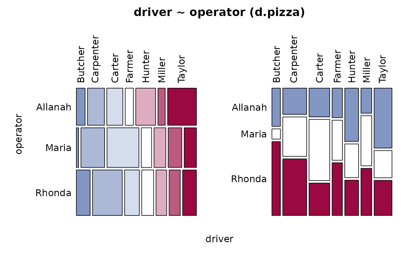 Desc(driver + area ~ operator, data=d.pizza) # several factors ~ factor
#> ──────────────────────────────────────────────────────────────────────────────
#> driver ~ operator (d.pizza)
#>
#> Summary:
#> n: 1'196, rows: 3, columns: 7
#>
#> Pearson's Chi-squared test:
#> X-squared = 133.06, df = 12, p-value < 2.2e-16
#> Log likelihood ratio (G-test) test of independence:
#> G = 133.53, X-squared df = 12, p-value < 2.2e-16
#> Mantel-Haenszel Chi-squared:
#> X-squared = 33.539, df = 1, p-value = 0.000000006984
#>
#> Contingency Coeff. 0.316
#> Cramer's V 0.236
#> Kendall Tau-b -0.145
#>
#>
#> driver Butcher Carpenter Carter Farmer Hunter Miller
#> operator
#>
#> Allanah freq 30 58 55 28 68 25
#> perc 2.5% 4.8% 4.6% 2.3% 5.7% 2.1%
#> p.row 8.3% 16.0% 15.2% 7.7% 18.7% 6.9%
#> p.col 31.2% 21.5% 23.5% 24.1% 43.6% 20.5%
#>
#> Maria freq 8 87 117 38 43 50
#> perc 0.7% 7.3% 9.8% 3.2% 3.6% 4.2%
#> p.row 2.1% 22.4% 30.2% 9.8% 11.1% 12.9%
#> p.col 8.3% 32.2% 50.0% 32.8% 27.6% 41.0%
#>
#> Rhonda freq 58 125 62 50 45 47
#> perc 4.8% 10.5% 5.2% 4.2% 3.8% 3.9%
#> p.row 13.0% 28.1% 13.9% 11.2% 10.1% 10.6%
#> p.col 60.4% 46.3% 26.5% 43.1% 28.8% 38.5%
#>
#> Sum freq 96 270 234 116 156 122
#> perc 8.0% 22.6% 19.6% 9.7% 13.0% 10.2%
#> p.row . . . . . .
#> p.col . . . . . .
#>
#>
#> driver Taylor Sum
#> operator
#>
#> Allanah freq 99 363
#> perc 8.3% 30.4%
#> p.row 27.3% .
#> p.col 49.0% .
#>
#> Maria freq 45 388
#> perc 3.8% 32.4%
#> p.row 11.6% .
#> p.col 22.3% .
#>
#> Rhonda freq 58 445
#> perc 4.8% 37.2%
#> p.row 13.0% .
#> p.col 28.7% .
#>
#> Sum freq 202 1'196
#> perc 16.9% 100.0%
#> p.row . .
#> p.col . .
#>
#>
#> ──────────────────────────────────────────────────────────────────────────────
#> area ~ operator (d.pizza)
#>
#> Summary:
#> n: 1'191, rows: 3, columns: 3
#>
#> Pearson's Chi-squared test:
#> X-squared = 17.905, df = 4, p-value = 0.001288
#> Log likelihood ratio (G-test) test of independence:
#> G = 18.099, X-squared df = 4, p-value = 0.001181
#> Mantel-Haenszel Chi-squared:
#> X-squared = 8.6654, df = 1, p-value = 0.003243
#>
#> Contingency Coeff. 0.122
#> Cramer's V 0.087
#> Kendall Tau-b 0.073
#>
#>
#> area Brent Camden Westminster Sum
#> operator
#>
#> Allanah freq 153 123 89 365
#> perc 12.8% 10.3% 7.5% 30.6%
#> p.row 41.9% 33.7% 24.4% .
#> p.col 32.3% 36.2% 23.5% .
#>
#> Maria freq 153 108 122 383
#> perc 12.8% 9.1% 10.2% 32.2%
#> p.row 39.9% 28.2% 31.9% .
#> p.col 32.3% 31.8% 32.3% .
#>
#> Rhonda freq 167 109 167 443
#> perc 14.0% 9.2% 14.0% 37.2%
#> p.row 37.7% 24.6% 37.7% .
#> p.col 35.3% 32.1% 44.2% .
#>
#> Sum freq 473 340 378 1'191
#> perc 39.7% 28.5% 31.7% 100.0%
#> p.row . . . .
#> p.col . . . .
#>
#>
Desc(driver + area ~ operator, data=d.pizza) # several factors ~ factor
#> ──────────────────────────────────────────────────────────────────────────────
#> driver ~ operator (d.pizza)
#>
#> Summary:
#> n: 1'196, rows: 3, columns: 7
#>
#> Pearson's Chi-squared test:
#> X-squared = 133.06, df = 12, p-value < 2.2e-16
#> Log likelihood ratio (G-test) test of independence:
#> G = 133.53, X-squared df = 12, p-value < 2.2e-16
#> Mantel-Haenszel Chi-squared:
#> X-squared = 33.539, df = 1, p-value = 0.000000006984
#>
#> Contingency Coeff. 0.316
#> Cramer's V 0.236
#> Kendall Tau-b -0.145
#>
#>
#> driver Butcher Carpenter Carter Farmer Hunter Miller
#> operator
#>
#> Allanah freq 30 58 55 28 68 25
#> perc 2.5% 4.8% 4.6% 2.3% 5.7% 2.1%
#> p.row 8.3% 16.0% 15.2% 7.7% 18.7% 6.9%
#> p.col 31.2% 21.5% 23.5% 24.1% 43.6% 20.5%
#>
#> Maria freq 8 87 117 38 43 50
#> perc 0.7% 7.3% 9.8% 3.2% 3.6% 4.2%
#> p.row 2.1% 22.4% 30.2% 9.8% 11.1% 12.9%
#> p.col 8.3% 32.2% 50.0% 32.8% 27.6% 41.0%
#>
#> Rhonda freq 58 125 62 50 45 47
#> perc 4.8% 10.5% 5.2% 4.2% 3.8% 3.9%
#> p.row 13.0% 28.1% 13.9% 11.2% 10.1% 10.6%
#> p.col 60.4% 46.3% 26.5% 43.1% 28.8% 38.5%
#>
#> Sum freq 96 270 234 116 156 122
#> perc 8.0% 22.6% 19.6% 9.7% 13.0% 10.2%
#> p.row . . . . . .
#> p.col . . . . . .
#>
#>
#> driver Taylor Sum
#> operator
#>
#> Allanah freq 99 363
#> perc 8.3% 30.4%
#> p.row 27.3% .
#> p.col 49.0% .
#>
#> Maria freq 45 388
#> perc 3.8% 32.4%
#> p.row 11.6% .
#> p.col 22.3% .
#>
#> Rhonda freq 58 445
#> perc 4.8% 37.2%
#> p.row 13.0% .
#> p.col 28.7% .
#>
#> Sum freq 202 1'196
#> perc 16.9% 100.0%
#> p.row . .
#> p.col . .
#>
#>
#> ──────────────────────────────────────────────────────────────────────────────
#> area ~ operator (d.pizza)
#>
#> Summary:
#> n: 1'191, rows: 3, columns: 3
#>
#> Pearson's Chi-squared test:
#> X-squared = 17.905, df = 4, p-value = 0.001288
#> Log likelihood ratio (G-test) test of independence:
#> G = 18.099, X-squared df = 4, p-value = 0.001181
#> Mantel-Haenszel Chi-squared:
#> X-squared = 8.6654, df = 1, p-value = 0.003243
#>
#> Contingency Coeff. 0.122
#> Cramer's V 0.087
#> Kendall Tau-b 0.073
#>
#>
#> area Brent Camden Westminster Sum
#> operator
#>
#> Allanah freq 153 123 89 365
#> perc 12.8% 10.3% 7.5% 30.6%
#> p.row 41.9% 33.7% 24.4% .
#> p.col 32.3% 36.2% 23.5% .
#>
#> Maria freq 153 108 122 383
#> perc 12.8% 9.1% 10.2% 32.2%
#> p.row 39.9% 28.2% 31.9% .
#> p.col 32.3% 31.8% 32.3% .
#>
#> Rhonda freq 167 109 167 443
#> perc 14.0% 9.2% 14.0% 37.2%
#> p.row 37.7% 24.6% 37.7% .
#> p.col 35.3% 32.1% 44.2% .
#>
#> Sum freq 473 340 378 1'191
#> perc 39.7% 28.5% 31.7% 100.0%
#> p.row . . . .
#> p.col . . . .
#>
#>
 Desc(driver ~ week, data=d.pizza) # factor ~ integer
#> ──────────────────────────────────────────────────────────────────────────────
#> driver ~ week (d.pizza)
#>
#> Summary:
#> n pairs: 1'209, valid: 1'172 (96.9%), missings: 37 (3.1%), groups: 7
#>
#>
#> Butcher Carpenter Carter Farmer Hunter Miller
#> mean 10.56989 11.82264 11.27876 11.52679 11.65806 11.60976
#> median 10.00000 12.00000 11.00000 11.00000 12.00000 12.00000
#> sd 1.12673 1.26231 1.24265 1.58233 1.24023 1.32216
#> IQR 2.00000 2.00000 2.00000 3.00000 2.00000 3.00000
#> n 93 265 226 112 155 123
#> np 7.93515% 22.61092% 19.28328% 9.55631% 13.22526% 10.49488%
#> NAs 3 7 8 5 1 2
#> 0s 0 0 0 0 0 0
#>
#> Taylor
#> mean 10.99495
#> median 11.00000
#> sd 1.21954
#> IQR 2.00000
#> n 198
#> np 16.89420%
#> NAs 6
#> 0s 0
#>
#> Kruskal-Wallis rank sum test:
#> Kruskal-Wallis chi-squared = 89.647, df = 6, p-value < 2.2e-16
#>
#>
#> Warning:
#> Grouping variable contains 5 NAs (0.414%).
#>
#>
#>
#> Proportions of driver in the quantiles of week:
#>
#> Q1 Q2 Q3 Q4
#> Butcher 13.7% 7.2% 5.1% 0.0%
#> Carpenter 15.5% 23.2% 25.0% 52.9%
#> Carter 22.4% 19.4% 17.5% 14.7%
#> Farmer 9.9% 9.9% 7.7% 32.4%
#> Hunter 8.7% 11.8% 17.7% 0.0%
#> Miller 9.9% 7.6% 13.0% 0.0%
#> Taylor 19.8% 20.9% 14.1% 0.0%
#>
Desc(driver ~ week, data=d.pizza) # factor ~ integer
#> ──────────────────────────────────────────────────────────────────────────────
#> driver ~ week (d.pizza)
#>
#> Summary:
#> n pairs: 1'209, valid: 1'172 (96.9%), missings: 37 (3.1%), groups: 7
#>
#>
#> Butcher Carpenter Carter Farmer Hunter Miller
#> mean 10.56989 11.82264 11.27876 11.52679 11.65806 11.60976
#> median 10.00000 12.00000 11.00000 11.00000 12.00000 12.00000
#> sd 1.12673 1.26231 1.24265 1.58233 1.24023 1.32216
#> IQR 2.00000 2.00000 2.00000 3.00000 2.00000 3.00000
#> n 93 265 226 112 155 123
#> np 7.93515% 22.61092% 19.28328% 9.55631% 13.22526% 10.49488%
#> NAs 3 7 8 5 1 2
#> 0s 0 0 0 0 0 0
#>
#> Taylor
#> mean 10.99495
#> median 11.00000
#> sd 1.21954
#> IQR 2.00000
#> n 198
#> np 16.89420%
#> NAs 6
#> 0s 0
#>
#> Kruskal-Wallis rank sum test:
#> Kruskal-Wallis chi-squared = 89.647, df = 6, p-value < 2.2e-16
#>
#>
#> Warning:
#> Grouping variable contains 5 NAs (0.414%).
#>
#>
#>
#> Proportions of driver in the quantiles of week:
#>
#> Q1 Q2 Q3 Q4
#> Butcher 13.7% 7.2% 5.1% 0.0%
#> Carpenter 15.5% 23.2% 25.0% 52.9%
#> Carter 22.4% 19.4% 17.5% 14.7%
#> Farmer 9.9% 9.9% 7.7% 32.4%
#> Hunter 8.7% 11.8% 17.7% 0.0%
#> Miller 9.9% 7.6% 13.0% 0.0%
#> Taylor 19.8% 20.9% 14.1% 0.0%
#>
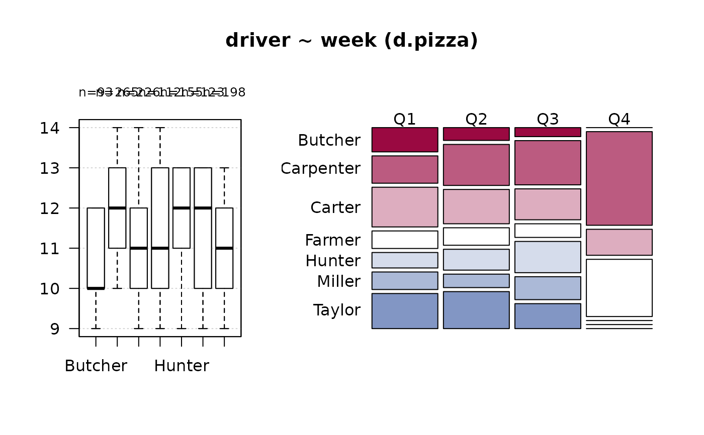 #> Warning: argument 1 does not name a graphical parameter
Desc(driver ~ operator, data=d.pizza, rfrq="111") # alle rel. frequencies
#> ──────────────────────────────────────────────────────────────────────────────
#> driver ~ operator (d.pizza)
#>
#> Summary:
#> n: 1'196, rows: 3, columns: 7
#>
#> Pearson's Chi-squared test:
#> X-squared = 133.06, df = 12, p-value < 2.2e-16
#> Log likelihood ratio (G-test) test of independence:
#> G = 133.53, X-squared df = 12, p-value < 2.2e-16
#> Mantel-Haenszel Chi-squared:
#> X-squared = 33.539, df = 1, p-value = 0.000000006984
#>
#> Contingency Coeff. 0.316
#> Cramer's V 0.236
#> Kendall Tau-b -0.145
#>
#>
#> driver Butcher Carpenter Carter Farmer Hunter Miller
#> operator
#>
#> Allanah freq 30 58 55 28 68 25
#> perc 2.5% 4.8% 4.6% 2.3% 5.7% 2.1%
#> p.row 8.3% 16.0% 15.2% 7.7% 18.7% 6.9%
#> p.col 31.2% 21.5% 23.5% 24.1% 43.6% 20.5%
#>
#> Maria freq 8 87 117 38 43 50
#> perc 0.7% 7.3% 9.8% 3.2% 3.6% 4.2%
#> p.row 2.1% 22.4% 30.2% 9.8% 11.1% 12.9%
#> p.col 8.3% 32.2% 50.0% 32.8% 27.6% 41.0%
#>
#> Rhonda freq 58 125 62 50 45 47
#> perc 4.8% 10.5% 5.2% 4.2% 3.8% 3.9%
#> p.row 13.0% 28.1% 13.9% 11.2% 10.1% 10.6%
#> p.col 60.4% 46.3% 26.5% 43.1% 28.8% 38.5%
#>
#> Sum freq 96 270 234 116 156 122
#> perc 8.0% 22.6% 19.6% 9.7% 13.0% 10.2%
#> p.row . . . . . .
#> p.col . . . . . .
#>
#>
#> driver Taylor Sum
#> operator
#>
#> Allanah freq 99 363
#> perc 8.3% 30.4%
#> p.row 27.3% .
#> p.col 49.0% .
#>
#> Maria freq 45 388
#> perc 3.8% 32.4%
#> p.row 11.6% .
#> p.col 22.3% .
#>
#> Rhonda freq 58 445
#> perc 4.8% 37.2%
#> p.row 13.0% .
#> p.col 28.7% .
#>
#> Sum freq 202 1'196
#> perc 16.9% 100.0%
#> p.row . .
#> p.col . .
#>
#>
#> Warning: argument 1 does not name a graphical parameter
Desc(driver ~ operator, data=d.pizza, rfrq="111") # alle rel. frequencies
#> ──────────────────────────────────────────────────────────────────────────────
#> driver ~ operator (d.pizza)
#>
#> Summary:
#> n: 1'196, rows: 3, columns: 7
#>
#> Pearson's Chi-squared test:
#> X-squared = 133.06, df = 12, p-value < 2.2e-16
#> Log likelihood ratio (G-test) test of independence:
#> G = 133.53, X-squared df = 12, p-value < 2.2e-16
#> Mantel-Haenszel Chi-squared:
#> X-squared = 33.539, df = 1, p-value = 0.000000006984
#>
#> Contingency Coeff. 0.316
#> Cramer's V 0.236
#> Kendall Tau-b -0.145
#>
#>
#> driver Butcher Carpenter Carter Farmer Hunter Miller
#> operator
#>
#> Allanah freq 30 58 55 28 68 25
#> perc 2.5% 4.8% 4.6% 2.3% 5.7% 2.1%
#> p.row 8.3% 16.0% 15.2% 7.7% 18.7% 6.9%
#> p.col 31.2% 21.5% 23.5% 24.1% 43.6% 20.5%
#>
#> Maria freq 8 87 117 38 43 50
#> perc 0.7% 7.3% 9.8% 3.2% 3.6% 4.2%
#> p.row 2.1% 22.4% 30.2% 9.8% 11.1% 12.9%
#> p.col 8.3% 32.2% 50.0% 32.8% 27.6% 41.0%
#>
#> Rhonda freq 58 125 62 50 45 47
#> perc 4.8% 10.5% 5.2% 4.2% 3.8% 3.9%
#> p.row 13.0% 28.1% 13.9% 11.2% 10.1% 10.6%
#> p.col 60.4% 46.3% 26.5% 43.1% 28.8% 38.5%
#>
#> Sum freq 96 270 234 116 156 122
#> perc 8.0% 22.6% 19.6% 9.7% 13.0% 10.2%
#> p.row . . . . . .
#> p.col . . . . . .
#>
#>
#> driver Taylor Sum
#> operator
#>
#> Allanah freq 99 363
#> perc 8.3% 30.4%
#> p.row 27.3% .
#> p.col 49.0% .
#>
#> Maria freq 45 388
#> perc 3.8% 32.4%
#> p.row 11.6% .
#> p.col 22.3% .
#>
#> Rhonda freq 58 445
#> perc 4.8% 37.2%
#> p.row 13.0% .
#> p.col 28.7% .
#>
#> Sum freq 202 1'196
#> perc 16.9% 100.0%
#> p.row . .
#> p.col . .
#>
#>
 Desc(driver ~ operator, data=d.pizza, rfrq="000",
verbose=3) # no rel. frequencies
#> ──────────────────────────────────────────────────────────────────────────────
#> driver ~ operator (d.pizza)
#>
#> Summary:
#> n: 1'196, rows: 3, columns: 7
#>
#> Pearson's Chi-squared test:
#> X-squared = 133.06, df = 12, p-value < 2.2e-16
#> Pearson's Chi-squared test (cont. adj):
#> X-squared = 133.06, df = 12, p-value < 2.2e-16
#> Log likelihood ratio (G-test) test of independence:
#> G = 133.53, X-squared df = 12, p-value < 2.2e-16
#> Mantel-Haenszel Chi-squared:
#> X-squared = 33.539, df = 1, p-value = 0.000000006984
#>
#> estimate lwr.ci upr.ci'
#> Contingency Coeff. 0.3164 - -
#> Cramer V 0.2359 0.1848 0.2668
#> Kendall Tau-b -0.1450 -0.1947 -0.0953
#> Goodman Kruskal Gamma -0.1923 -0.2579 -0.1268
#> Stuart Tau-c -0.1624 -0.2180 -0.1067
#> Somers D C|R -0.1630 -0.2188 -0.1071
#> Somers D R|C -0.1290 -0.1734 -0.0846
#> Pearson Correlation -0.1675 -0.2221 -0.1119
#> Spearman Correlation -0.1706 -0.2251 -0.1150
#> Lambda C|R 0.0767 0.0380 0.1153
#> Lambda R|C 0.1625 0.1066 0.2183
#> Lambda sym 0.1151 0.0745 0.1557
#> Uncertainty Coeff. C|R 0.0296 0.0199 0.0394
#> Uncertainty Coeff. R|C 0.0510 0.0342 0.0677
#> Uncertainty Coeff. sym 0.0375 0.0252 0.0498
#> Mutual Information 0.0805 - -
#>
#>
#> driver Butcher Carpenter Carter Farmer Hunter Miller Taylor
#> operator
#> Allanah 30 58 55 28 68 25 99
#> Maria 8 87 117 38 43 50 45
#> Rhonda 58 125 62 50 45 47 58
#> Sum 96 270 234 116 156 122 202
#>
#> driver Sum
#> operator
#> Allanah 363
#> Maria 388
#> Rhonda 445
#> Sum 1'196
#>
#> ────────────────────
#> ' 95% conf. level
#>
Desc(price ~ delivery_min, data=d.pizza) # numeric ~ numeric
#> ──────────────────────────────────────────────────────────────────────────────
#> price ~ delivery_min (d.pizza)
#>
#> Summary:
#> n pairs: 1'209, valid: 1'197 (99.0%), missings: 12 (1.0%)
#>
#>
#> Pearson corr. : 0.095
#> Spearman corr.: 0.080
#> Kendall corr. : 0.054
#>
Desc(driver ~ operator, data=d.pizza, rfrq="000",
verbose=3) # no rel. frequencies
#> ──────────────────────────────────────────────────────────────────────────────
#> driver ~ operator (d.pizza)
#>
#> Summary:
#> n: 1'196, rows: 3, columns: 7
#>
#> Pearson's Chi-squared test:
#> X-squared = 133.06, df = 12, p-value < 2.2e-16
#> Pearson's Chi-squared test (cont. adj):
#> X-squared = 133.06, df = 12, p-value < 2.2e-16
#> Log likelihood ratio (G-test) test of independence:
#> G = 133.53, X-squared df = 12, p-value < 2.2e-16
#> Mantel-Haenszel Chi-squared:
#> X-squared = 33.539, df = 1, p-value = 0.000000006984
#>
#> estimate lwr.ci upr.ci'
#> Contingency Coeff. 0.3164 - -
#> Cramer V 0.2359 0.1848 0.2668
#> Kendall Tau-b -0.1450 -0.1947 -0.0953
#> Goodman Kruskal Gamma -0.1923 -0.2579 -0.1268
#> Stuart Tau-c -0.1624 -0.2180 -0.1067
#> Somers D C|R -0.1630 -0.2188 -0.1071
#> Somers D R|C -0.1290 -0.1734 -0.0846
#> Pearson Correlation -0.1675 -0.2221 -0.1119
#> Spearman Correlation -0.1706 -0.2251 -0.1150
#> Lambda C|R 0.0767 0.0380 0.1153
#> Lambda R|C 0.1625 0.1066 0.2183
#> Lambda sym 0.1151 0.0745 0.1557
#> Uncertainty Coeff. C|R 0.0296 0.0199 0.0394
#> Uncertainty Coeff. R|C 0.0510 0.0342 0.0677
#> Uncertainty Coeff. sym 0.0375 0.0252 0.0498
#> Mutual Information 0.0805 - -
#>
#>
#> driver Butcher Carpenter Carter Farmer Hunter Miller Taylor
#> operator
#> Allanah 30 58 55 28 68 25 99
#> Maria 8 87 117 38 43 50 45
#> Rhonda 58 125 62 50 45 47 58
#> Sum 96 270 234 116 156 122 202
#>
#> driver Sum
#> operator
#> Allanah 363
#> Maria 388
#> Rhonda 445
#> Sum 1'196
#>
#> ────────────────────
#> ' 95% conf. level
#>
Desc(price ~ delivery_min, data=d.pizza) # numeric ~ numeric
#> ──────────────────────────────────────────────────────────────────────────────
#> price ~ delivery_min (d.pizza)
#>
#> Summary:
#> n pairs: 1'209, valid: 1'197 (99.0%), missings: 12 (1.0%)
#>
#>
#> Pearson corr. : 0.095
#> Spearman corr.: 0.080
#> Kendall corr. : 0.054
#>
 Desc(price + delivery_min ~ operator + driver + wrongpizza,
data=d.pizza, digits=c(2,2,2,2,0,3,0,0) )
#> ──────────────────────────────────────────────────────────────────────────────
#> price ~ operator (d.pizza)
#>
#> Summary:
#> n pairs: 1'209, valid: 1'189 (98.3%), missings: 20 (1.7%), groups: 3
#>
#>
#> Allanah Maria Rhonda
#> mean 46.31 49.12 50.37
#> median 44.97 46.76 47.97
#> sd 20.15 21.98 22.41
#> IQR 28.87 31.83 33.43
#> n 363 384 442
#> np 31% 32% 37%
#> NAs 4 4 4
#> 0s 0 0 0
#>
#> Kruskal-Wallis rank sum test:
#> Kruskal-Wallis chi-squared = 6.2048, df = 2, p-value = 0.04494
#>
#>
#> Warning:
#> Grouping variable contains 8 NAs (0.662%).
#>
Desc(price + delivery_min ~ operator + driver + wrongpizza,
data=d.pizza, digits=c(2,2,2,2,0,3,0,0) )
#> ──────────────────────────────────────────────────────────────────────────────
#> price ~ operator (d.pizza)
#>
#> Summary:
#> n pairs: 1'209, valid: 1'189 (98.3%), missings: 20 (1.7%), groups: 3
#>
#>
#> Allanah Maria Rhonda
#> mean 46.31 49.12 50.37
#> median 44.97 46.76 47.97
#> sd 20.15 21.98 22.41
#> IQR 28.87 31.83 33.43
#> n 363 384 442
#> np 31% 32% 37%
#> NAs 4 4 4
#> 0s 0 0 0
#>
#> Kruskal-Wallis rank sum test:
#> Kruskal-Wallis chi-squared = 6.2048, df = 2, p-value = 0.04494
#>
#>
#> Warning:
#> Grouping variable contains 8 NAs (0.662%).
#>
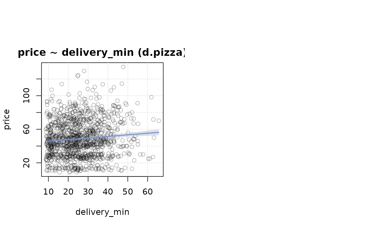 #> ──────────────────────────────────────────────────────────────────────────────
#> price ~ driver (d.pizza)
#>
#> Summary:
#> n pairs: 1'209, valid: 1'192 (98.6%), missings: 17 (1.4%), groups: 7
#>
#>
#> Butcher Carpenter Carter Farmer Hunter Miller
#> mean 45.88 54.19 45.45 49.50 44.29 50.02
#> median 44.97 50.36 43.97 47.66 42.71 46.97
#> sd 20.74 24.23 21.66 18.53 19.67 21.32
#> IQR 27.88 32.68 32.28 20.39 23.98 35.57
#> n 94 270 231 117 154 125
#> np 8% 23% 19% 10% 13% 10%
#> NAs 2 2 3 0 2 0
#> 0s 0 0 0 0 0 0
#>
#> Taylor
#> mean 48.46
#> median 46.97
#> sd 19.97
#> IQR 28.99
#> n 201
#> np 17%
#> NAs 3
#> 0s 0
#>
#> Kruskal-Wallis rank sum test:
#> Kruskal-Wallis chi-squared = 26.137, df = 6, p-value = 0.0002099
#>
#>
#> Warning:
#> Grouping variable contains 5 NAs (0.414%).
#>
#> ──────────────────────────────────────────────────────────────────────────────
#> price ~ driver (d.pizza)
#>
#> Summary:
#> n pairs: 1'209, valid: 1'192 (98.6%), missings: 17 (1.4%), groups: 7
#>
#>
#> Butcher Carpenter Carter Farmer Hunter Miller
#> mean 45.88 54.19 45.45 49.50 44.29 50.02
#> median 44.97 50.36 43.97 47.66 42.71 46.97
#> sd 20.74 24.23 21.66 18.53 19.67 21.32
#> IQR 27.88 32.68 32.28 20.39 23.98 35.57
#> n 94 270 231 117 154 125
#> np 8% 23% 19% 10% 13% 10%
#> NAs 2 2 3 0 2 0
#> 0s 0 0 0 0 0 0
#>
#> Taylor
#> mean 48.46
#> median 46.97
#> sd 19.97
#> IQR 28.99
#> n 201
#> np 17%
#> NAs 3
#> 0s 0
#>
#> Kruskal-Wallis rank sum test:
#> Kruskal-Wallis chi-squared = 26.137, df = 6, p-value = 0.0002099
#>
#>
#> Warning:
#> Grouping variable contains 5 NAs (0.414%).
#>
 #> ──────────────────────────────────────────────────────────────────────────────
#> price ~ wrongpizza (d.pizza)
#>
#> Summary:
#> n pairs: 1'209, valid: 1'193 (98.7%), missings: 16 (1.3%), groups: 2
#>
#>
#> FALSE TRUE
#> mean 48.57 51.41
#> median 46.76 48.56
#> sd 21.60 22.21
#> IQR 32.09 34.05
#> n 1'111 82
#> np 93% 7%
#> NAs 11 1
#> 0s 0 0
#>
#> Kruskal-Wallis rank sum test:
#> Kruskal-Wallis chi-squared = 1.2512, df = 1, p-value = 0.2633
#>
#>
#> Warning:
#> Grouping variable contains 4 NAs (0.331%).
#>
#> ──────────────────────────────────────────────────────────────────────────────
#> price ~ wrongpizza (d.pizza)
#>
#> Summary:
#> n pairs: 1'209, valid: 1'193 (98.7%), missings: 16 (1.3%), groups: 2
#>
#>
#> FALSE TRUE
#> mean 48.57 51.41
#> median 46.76 48.56
#> sd 21.60 22.21
#> IQR 32.09 34.05
#> n 1'111 82
#> np 93% 7%
#> NAs 11 1
#> 0s 0 0
#>
#> Kruskal-Wallis rank sum test:
#> Kruskal-Wallis chi-squared = 1.2512, df = 1, p-value = 0.2633
#>
#>
#> Warning:
#> Grouping variable contains 4 NAs (0.331%).
#>
 #> ──────────────────────────────────────────────────────────────────────────────
#> delivery_min ~ operator (d.pizza)
#>
#> Summary:
#> n pairs: 1'209, valid: 1'201 (99.3%), missings: 8 (0.7%), groups: 3
#>
#>
#> Allanah Maria Rhonda
#> mean 23.82 26.90 26.06
#> median 22.70 25.65 24.75
#> sd 10.34 11.06 10.86
#> IQR 15.55 15.18 14.88
#> n 367 388 446
#> np 31% 32% 37%
#> NAs 0 0 0
#> 0s 0 0 0
#>
#> Kruskal-Wallis rank sum test:
#> Kruskal-Wallis chi-squared = 15.847, df = 2, p-value = 0.0003622
#>
#>
#> Warning:
#> Grouping variable contains 8 NAs (0.662%).
#>
#> ──────────────────────────────────────────────────────────────────────────────
#> delivery_min ~ operator (d.pizza)
#>
#> Summary:
#> n pairs: 1'209, valid: 1'201 (99.3%), missings: 8 (0.7%), groups: 3
#>
#>
#> Allanah Maria Rhonda
#> mean 23.82 26.90 26.06
#> median 22.70 25.65 24.75
#> sd 10.34 11.06 10.86
#> IQR 15.55 15.18 14.88
#> n 367 388 446
#> np 31% 32% 37%
#> NAs 0 0 0
#> 0s 0 0 0
#>
#> Kruskal-Wallis rank sum test:
#> Kruskal-Wallis chi-squared = 15.847, df = 2, p-value = 0.0003622
#>
#>
#> Warning:
#> Grouping variable contains 8 NAs (0.662%).
#>
 #> ──────────────────────────────────────────────────────────────────────────────
#> delivery_min ~ driver (d.pizza)
#>
#> Summary:
#> n pairs: 1'209, valid: 1'204 (99.6%), missings: 5 (0.4%), groups: 7
#>
#>
#> Butcher Carpenter Carter Farmer Hunter Miller
#> mean 18.88 32.73 24.41 20.15 18.51 25.55
#> median 16.85 32.85 24.00 19.20 16.65 24.90
#> sd 9.41 11.28 8.84 7.41 8.37 8.80
#> IQR 14.40 15.12 11.82 9.60 10.53 10.80
#> n 96 272 234 117 156 125
#> np 8% 23% 19% 10% 13% 10%
#> NAs 0 0 0 0 0 0
#> 0s 0 0 0 0 0 0
#>
#> Taylor
#> mean 29.52
#> median 28.20
#> sd 10.13
#> IQR 13.85
#> n 204
#> np 17%
#> NAs 0
#> 0s 0
#>
#> Kruskal-Wallis rank sum test:
#> Kruskal-Wallis chi-squared = 289.47, df = 6, p-value < 2.2e-16
#>
#>
#> Warning:
#> Grouping variable contains 5 NAs (0.414%).
#>
#> ──────────────────────────────────────────────────────────────────────────────
#> delivery_min ~ driver (d.pizza)
#>
#> Summary:
#> n pairs: 1'209, valid: 1'204 (99.6%), missings: 5 (0.4%), groups: 7
#>
#>
#> Butcher Carpenter Carter Farmer Hunter Miller
#> mean 18.88 32.73 24.41 20.15 18.51 25.55
#> median 16.85 32.85 24.00 19.20 16.65 24.90
#> sd 9.41 11.28 8.84 7.41 8.37 8.80
#> IQR 14.40 15.12 11.82 9.60 10.53 10.80
#> n 96 272 234 117 156 125
#> np 8% 23% 19% 10% 13% 10%
#> NAs 0 0 0 0 0 0
#> 0s 0 0 0 0 0 0
#>
#> Taylor
#> mean 29.52
#> median 28.20
#> sd 10.13
#> IQR 13.85
#> n 204
#> np 17%
#> NAs 0
#> 0s 0
#>
#> Kruskal-Wallis rank sum test:
#> Kruskal-Wallis chi-squared = 289.47, df = 6, p-value < 2.2e-16
#>
#>
#> Warning:
#> Grouping variable contains 5 NAs (0.414%).
#>
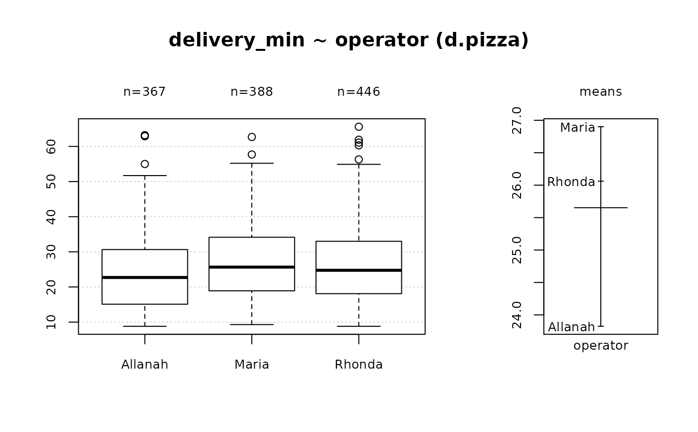 #> ──────────────────────────────────────────────────────────────────────────────
#> delivery_min ~ wrongpizza (d.pizza)
#>
#> Summary:
#> n pairs: 1'209, valid: 1'205 (99.7%), missings: 4 (0.3%), groups: 2
#>
#>
#> FALSE TRUE
#> mean 25.62 26.11
#> median 24.35 25.30
#> sd 10.87 10.60
#> IQR 15.07 15.10
#> n 1'122 83
#> np 93% 7%
#> NAs 0 0
#> 0s 0 0
#>
#> Kruskal-Wallis rank sum test:
#> Kruskal-Wallis chi-squared = 0.36826, df = 1, p-value = 0.544
#>
#>
#> Warning:
#> Grouping variable contains 4 NAs (0.331%).
#>
#> ──────────────────────────────────────────────────────────────────────────────
#> delivery_min ~ wrongpizza (d.pizza)
#>
#> Summary:
#> n pairs: 1'209, valid: 1'205 (99.7%), missings: 4 (0.3%), groups: 2
#>
#>
#> FALSE TRUE
#> mean 25.62 26.11
#> median 24.35 25.30
#> sd 10.87 10.60
#> IQR 15.07 15.10
#> n 1'122 83
#> np 93% 7%
#> NAs 0 0
#> 0s 0 0
#>
#> Kruskal-Wallis rank sum test:
#> Kruskal-Wallis chi-squared = 0.36826, df = 1, p-value = 0.544
#>
#>
#> Warning:
#> Grouping variable contains 4 NAs (0.331%).
#>
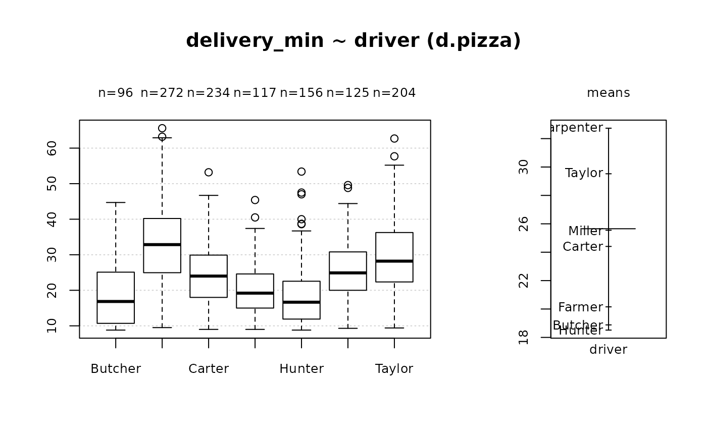 Desc(week ~ driver, data=d.pizza, digits=c(2,2,2,2,0,3,0,0)) # define digits
#> ──────────────────────────────────────────────────────────────────────────────
#> week ~ driver (d.pizza)
#>
#> Summary:
#> n pairs: 1'209, valid: 1'172 (96.9%), missings: 37 (3.1%), groups: 7
#>
#>
#> Butcher Carpenter Carter Farmer Hunter Miller
#> mean 10.57 11.82 11.28 11.53 11.66 11.61
#> median 10.00 12.00 11.00 11.00 12.00 12.00
#> sd 1.13 1.26 1.24 1.58 1.24 1.32
#> IQR 2.00 2.00 2.00 3.00 2.00 3.00
#> n 93 265 226 112 155 123
#> np 8% 23% 19% 10% 13% 10%
#> NAs 3 7 8 5 1 2
#> 0s 0 0 0 0 0 0
#>
#> Taylor
#> mean 10.99
#> median 11.00
#> sd 1.22
#> IQR 2.00
#> n 198
#> np 17%
#> NAs 6
#> 0s 0
#>
#> Kruskal-Wallis rank sum test:
#> Kruskal-Wallis chi-squared = 89.647, df = 6, p-value < 2.2e-16
#>
#>
#> Warning:
#> Grouping variable contains 5 NAs (0.414%).
#>
Desc(week ~ driver, data=d.pizza, digits=c(2,2,2,2,0,3,0,0)) # define digits
#> ──────────────────────────────────────────────────────────────────────────────
#> week ~ driver (d.pizza)
#>
#> Summary:
#> n pairs: 1'209, valid: 1'172 (96.9%), missings: 37 (3.1%), groups: 7
#>
#>
#> Butcher Carpenter Carter Farmer Hunter Miller
#> mean 10.57 11.82 11.28 11.53 11.66 11.61
#> median 10.00 12.00 11.00 11.00 12.00 12.00
#> sd 1.13 1.26 1.24 1.58 1.24 1.32
#> IQR 2.00 2.00 2.00 3.00 2.00 3.00
#> n 93 265 226 112 155 123
#> np 8% 23% 19% 10% 13% 10%
#> NAs 3 7 8 5 1 2
#> 0s 0 0 0 0 0 0
#>
#> Taylor
#> mean 10.99
#> median 11.00
#> sd 1.22
#> IQR 2.00
#> n 198
#> np 17%
#> NAs 6
#> 0s 0
#>
#> Kruskal-Wallis rank sum test:
#> Kruskal-Wallis chi-squared = 89.647, df = 6, p-value < 2.2e-16
#>
#>
#> Warning:
#> Grouping variable contains 5 NAs (0.414%).
#>
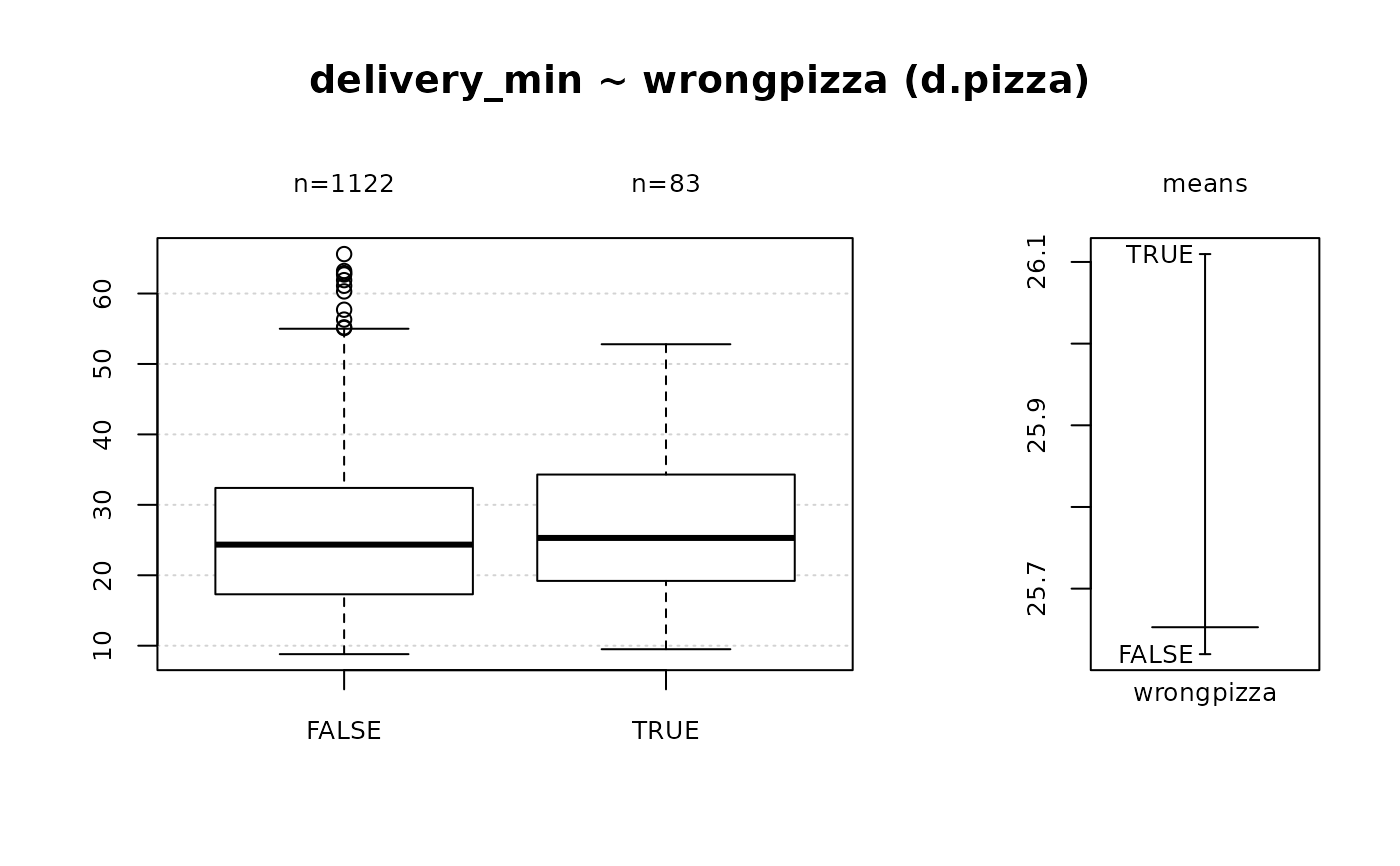 Desc(delivery_min + weekday ~ driver, data=d.pizza)
#> ──────────────────────────────────────────────────────────────────────────────
#> delivery_min ~ driver (d.pizza)
#>
#> Summary:
#> n pairs: 1'209, valid: 1'204 (99.6%), missings: 5 (0.4%), groups: 7
#>
#>
#> Butcher Carpenter Carter Farmer Hunter Miller
#> mean 18.88125 32.73235 24.40684 20.15214 18.51474 25.54720
#> median 16.85000 32.85000 24.00000 19.20000 16.65000 24.90000
#> sd 9.40621 11.28065 8.84066 7.40856 8.37358 8.80189
#> IQR 14.40000 15.12500 11.82500 9.60000 10.52500 10.80000
#> n 96 272 234 117 156 125
#> np 7.97342% 22.59136% 19.43522% 9.71761% 12.95681% 10.38206%
#> NAs 0 0 0 0 0 0
#> 0s 0 0 0 0 0 0
#>
#> Taylor
#> mean 29.52402
#> median 28.20000
#> sd 10.13141
#> IQR 13.85000
#> n 204
#> np 16.94352%
#> NAs 0
#> 0s 0
#>
#> Kruskal-Wallis rank sum test:
#> Kruskal-Wallis chi-squared = 289.47, df = 6, p-value < 2.2e-16
#>
#>
#> Warning:
#> Grouping variable contains 5 NAs (0.414%).
#>
Desc(delivery_min + weekday ~ driver, data=d.pizza)
#> ──────────────────────────────────────────────────────────────────────────────
#> delivery_min ~ driver (d.pizza)
#>
#> Summary:
#> n pairs: 1'209, valid: 1'204 (99.6%), missings: 5 (0.4%), groups: 7
#>
#>
#> Butcher Carpenter Carter Farmer Hunter Miller
#> mean 18.88125 32.73235 24.40684 20.15214 18.51474 25.54720
#> median 16.85000 32.85000 24.00000 19.20000 16.65000 24.90000
#> sd 9.40621 11.28065 8.84066 7.40856 8.37358 8.80189
#> IQR 14.40000 15.12500 11.82500 9.60000 10.52500 10.80000
#> n 96 272 234 117 156 125
#> np 7.97342% 22.59136% 19.43522% 9.71761% 12.95681% 10.38206%
#> NAs 0 0 0 0 0 0
#> 0s 0 0 0 0 0 0
#>
#> Taylor
#> mean 29.52402
#> median 28.20000
#> sd 10.13141
#> IQR 13.85000
#> n 204
#> np 16.94352%
#> NAs 0
#> 0s 0
#>
#> Kruskal-Wallis rank sum test:
#> Kruskal-Wallis chi-squared = 289.47, df = 6, p-value < 2.2e-16
#>
#>
#> Warning:
#> Grouping variable contains 5 NAs (0.414%).
#>
 #> ──────────────────────────────────────────────────────────────────────────────
#> weekday ~ driver (d.pizza)
#>
#> Summary:
#> n pairs: 1'209, valid: 1'172 (96.9%), missings: 37 (3.1%), groups: 7
#>
#>
#> Butcher Carpenter Carter Farmer Hunter Miller
#> mean 6.47312 4.70943 3.80531 3.83036 3.90323 5.01626
#> median 6.00000 5.00000 4.00000 4.00000 3.00000 5.00000
#> sd 0.50198 1.97391 1.57400 1.75985 2.39256 1.45975
#> IQR 1.00000 2.00000 2.75000 2.00000 5.00000 1.50000
#> n 93 265 226 112 155 123
#> np 7.93515% 22.61092% 19.28328% 9.55631% 13.22526% 10.49488%
#> NAs 3 7 8 5 1 2
#> 0s 0 0 0 0 0 0
#>
#> Taylor
#> mean 4.29798
#> median 6.00000
#> sd 2.29922
#> IQR 4.00000
#> n 198
#> np 16.89420%
#> NAs 6
#> 0s 0
#>
#> Kruskal-Wallis rank sum test:
#> Kruskal-Wallis chi-squared = 164.67, df = 6, p-value < 2.2e-16
#>
#>
#> Warning:
#> Grouping variable contains 5 NAs (0.414%).
#>
#> ──────────────────────────────────────────────────────────────────────────────
#> weekday ~ driver (d.pizza)
#>
#> Summary:
#> n pairs: 1'209, valid: 1'172 (96.9%), missings: 37 (3.1%), groups: 7
#>
#>
#> Butcher Carpenter Carter Farmer Hunter Miller
#> mean 6.47312 4.70943 3.80531 3.83036 3.90323 5.01626
#> median 6.00000 5.00000 4.00000 4.00000 3.00000 5.00000
#> sd 0.50198 1.97391 1.57400 1.75985 2.39256 1.45975
#> IQR 1.00000 2.00000 2.75000 2.00000 5.00000 1.50000
#> n 93 265 226 112 155 123
#> np 7.93515% 22.61092% 19.28328% 9.55631% 13.22526% 10.49488%
#> NAs 3 7 8 5 1 2
#> 0s 0 0 0 0 0 0
#>
#> Taylor
#> mean 4.29798
#> median 6.00000
#> sd 2.29922
#> IQR 4.00000
#> n 198
#> np 16.89420%
#> NAs 6
#> 0s 0
#>
#> Kruskal-Wallis rank sum test:
#> Kruskal-Wallis chi-squared = 164.67, df = 6, p-value < 2.2e-16
#>
#>
#> Warning:
#> Grouping variable contains 5 NAs (0.414%).
#>
 # without defining data-parameter
Desc(d.pizza$delivery_min ~ d.pizza$driver)
#> ──────────────────────────────────────────────────────────────────────────────
#> d.pizza$delivery_min ~ d.pizza$driver
#>
#> Summary:
#> n pairs: 1'209, valid: 1'204 (99.6%), missings: 5 (0.4%), groups: 7
#>
#>
#> Butcher Carpenter Carter Farmer Hunter Miller
#> mean 18.88125 32.73235 24.40684 20.15214 18.51474 25.54720
#> median 16.85000 32.85000 24.00000 19.20000 16.65000 24.90000
#> sd 9.40621 11.28065 8.84066 7.40856 8.37358 8.80189
#> IQR 14.40000 15.12500 11.82500 9.60000 10.52500 10.80000
#> n 96 272 234 117 156 125
#> np 7.97342% 22.59136% 19.43522% 9.71761% 12.95681% 10.38206%
#> NAs 0 0 0 0 0 0
#> 0s 0 0 0 0 0 0
#>
#> Taylor
#> mean 29.52402
#> median 28.20000
#> sd 10.13141
#> IQR 13.85000
#> n 204
#> np 16.94352%
#> NAs 0
#> 0s 0
#>
#> Kruskal-Wallis rank sum test:
#> Kruskal-Wallis chi-squared = 289.47, df = 6, p-value < 2.2e-16
#>
#>
#> Warning:
#> Grouping variable contains 5 NAs (0.414%).
#>
# without defining data-parameter
Desc(d.pizza$delivery_min ~ d.pizza$driver)
#> ──────────────────────────────────────────────────────────────────────────────
#> d.pizza$delivery_min ~ d.pizza$driver
#>
#> Summary:
#> n pairs: 1'209, valid: 1'204 (99.6%), missings: 5 (0.4%), groups: 7
#>
#>
#> Butcher Carpenter Carter Farmer Hunter Miller
#> mean 18.88125 32.73235 24.40684 20.15214 18.51474 25.54720
#> median 16.85000 32.85000 24.00000 19.20000 16.65000 24.90000
#> sd 9.40621 11.28065 8.84066 7.40856 8.37358 8.80189
#> IQR 14.40000 15.12500 11.82500 9.60000 10.52500 10.80000
#> n 96 272 234 117 156 125
#> np 7.97342% 22.59136% 19.43522% 9.71761% 12.95681% 10.38206%
#> NAs 0 0 0 0 0 0
#> 0s 0 0 0 0 0 0
#>
#> Taylor
#> mean 29.52402
#> median 28.20000
#> sd 10.13141
#> IQR 13.85000
#> n 204
#> np 16.94352%
#> NAs 0
#> 0s 0
#>
#> Kruskal-Wallis rank sum test:
#> Kruskal-Wallis chi-squared = 289.47, df = 6, p-value < 2.2e-16
#>
#>
#> Warning:
#> Grouping variable contains 5 NAs (0.414%).
#>
 # with functions and interactions
Desc(sqrt(price) ~ operator : factor(wrongpizza), data=d.pizza)
#> ──────────────────────────────────────────────────────────────────────────────
#> sqrt(price) ~ operator:factor(wrongpizza) (d.pizza)
#>
#> Summary:
#> n pairs: 1'209, valid: 1'185 (98.0%), missings: 24 (2.0%), groups: 6
#>
#>
#> Allanah:FALSE Maria:FALSE Rhonda:FALSE Allanah:TRUE
#> mean 6.62506 6.79423 6.91301 7.23357
#> median 6.70597 6.78012 6.92965 7.46194
#> sd 1.53011 1.57618 1.64992 1.28011
#> IQR 2.19071 2.29395 2.50547 0.93878
#> n 359 313 432 4
#> np 30.29536% 26.41350% 36.45570% 0.33755%
#> NAs 4 3 4 0
#> 0s 0 0 0 0
#>
#> Maria:TRUE Rhonda:TRUE
#> mean 7.02072 6.50934
#> median 6.96879 6.81679
#> sd 1.63467 1.46372
#> IQR 2.64658 1.06284
#> n 69 8
#> np 5.82278% 0.67511%
#> NAs 1 0
#> 0s 0 0
#>
#> Kruskal-Wallis rank sum test:
#> Kruskal-Wallis chi-squared = 8.5064, df = 5, p-value = 0.1304
#>
#>
#> Warning:
#> Grouping variable contains 12 NAs (0.993%).
#>
# with functions and interactions
Desc(sqrt(price) ~ operator : factor(wrongpizza), data=d.pizza)
#> ──────────────────────────────────────────────────────────────────────────────
#> sqrt(price) ~ operator:factor(wrongpizza) (d.pizza)
#>
#> Summary:
#> n pairs: 1'209, valid: 1'185 (98.0%), missings: 24 (2.0%), groups: 6
#>
#>
#> Allanah:FALSE Maria:FALSE Rhonda:FALSE Allanah:TRUE
#> mean 6.62506 6.79423 6.91301 7.23357
#> median 6.70597 6.78012 6.92965 7.46194
#> sd 1.53011 1.57618 1.64992 1.28011
#> IQR 2.19071 2.29395 2.50547 0.93878
#> n 359 313 432 4
#> np 30.29536% 26.41350% 36.45570% 0.33755%
#> NAs 4 3 4 0
#> 0s 0 0 0 0
#>
#> Maria:TRUE Rhonda:TRUE
#> mean 7.02072 6.50934
#> median 6.96879 6.81679
#> sd 1.63467 1.46372
#> IQR 2.64658 1.06284
#> n 69 8
#> np 5.82278% 0.67511%
#> NAs 1 0
#> 0s 0 0
#>
#> Kruskal-Wallis rank sum test:
#> Kruskal-Wallis chi-squared = 8.5064, df = 5, p-value = 0.1304
#>
#>
#> Warning:
#> Grouping variable contains 12 NAs (0.993%).
#>
 Desc(log(price+1) ~ cut(delivery_min, breaks=seq(10,90,10)),
data=d.pizza, digits=c(2,2,2,2,0,3,0,0))
#> ──────────────────────────────────────────────────────────────────────────────
#> log(price + 1) ~ cut(delivery_min, breaks = seq(10, 90, 10)) (d.pizza)
#>
#> Summary:
#> n pairs: 1'209, valid: 1'147 (94.9%), missings: 62 (5.1%), groups: 6
#>
#>
#> (10,20] (20,30] (30,40] (40,50] (50,60] (60,70]
#> mean 3.77 3.80 3.81 3.90 3.84 3.85
#> median 3.83 3.87 3.87 4.01 3.89 3.93
#> sd 0.46 0.51 0.48 0.56 0.44 0.56
#> IQR 0.65 0.68 0.68 0.70 0.73 0.98
#> n 346 427 245 98 24 7
#> np 30% 37% 21% 9% 2% 1%
#> NAs 5 3 3 1 0 0
#> 0s 0 0 0 0 0 0
#>
#> Kruskal-Wallis rank sum test:
#> Kruskal-Wallis chi-squared = 8.1513, df = 5, p-value = 0.1481
#>
#>
#> Warning:
#> Grouping variable contains 50 NAs (4.14%).
#>
Desc(log(price+1) ~ cut(delivery_min, breaks=seq(10,90,10)),
data=d.pizza, digits=c(2,2,2,2,0,3,0,0))
#> ──────────────────────────────────────────────────────────────────────────────
#> log(price + 1) ~ cut(delivery_min, breaks = seq(10, 90, 10)) (d.pizza)
#>
#> Summary:
#> n pairs: 1'209, valid: 1'147 (94.9%), missings: 62 (5.1%), groups: 6
#>
#>
#> (10,20] (20,30] (30,40] (40,50] (50,60] (60,70]
#> mean 3.77 3.80 3.81 3.90 3.84 3.85
#> median 3.83 3.87 3.87 4.01 3.89 3.93
#> sd 0.46 0.51 0.48 0.56 0.44 0.56
#> IQR 0.65 0.68 0.68 0.70 0.73 0.98
#> n 346 427 245 98 24 7
#> np 30% 37% 21% 9% 2% 1%
#> NAs 5 3 3 1 0 0
#> 0s 0 0 0 0 0 0
#>
#> Kruskal-Wallis rank sum test:
#> Kruskal-Wallis chi-squared = 8.1513, df = 5, p-value = 0.1481
#>
#>
#> Warning:
#> Grouping variable contains 50 NAs (4.14%).
#>
 # response versus all the rest
Desc(driver ~ ., data=d.pizza[, c("temperature","wine_delivered","area","driver")])
#> ──────────────────────────────────────────────────────────────────────────────
#> driver ~ temperature (d.pizza[, c("temperature", "wine_delivered", "area", "driver")])
#>
#> Summary:
#> n pairs: 1'209, valid: 1'166 (96.4%), missings: 43 (3.6%), groups: 7
#>
#>
#> Butcher Carpenter Carter Farmer Hunter Miller
#> mean 49.61719 43.49348 50.41925 50.93675 52.14135 47.52397
#> median 51.40000 44.80000 51.75000 54.10000 55.10000 49.60000
#> sd 8.78704 9.40667 8.46700 9.02373 8.88544 8.93474
#> IQR 11.97500 12.50000 11.32500 11.20000 11.57500 8.80000
#> n 96 253 226 117 156 121
#> np 8.23328% 21.69811% 19.38250% 10.03431% 13.37907% 10.37736%
#> NAs 0 19 8 0 0 4
#> 0s 0 0 0 0 0 0
#>
#> Taylor
#> mean 45.09061
#> median 48.50000
#> sd 11.44201
#> IQR 18.40000
#> n 197
#> np 16.89537%
#> NAs 7
#> 0s 0
#>
#> Kruskal-Wallis rank sum test:
#> Kruskal-Wallis chi-squared = 141.93, df = 6, p-value < 2.2e-16
#>
#>
#> Warning:
#> Grouping variable contains 5 NAs (0.414%).
#>
#>
#>
#> Proportions of driver in the quantiles of temperature:
#>
#> Q1 Q2 Q3 Q4
#> Butcher 6.8% 8.1% 7.3% 10.7%
#> Carpenter 34.9% 28.8% 15.9% 6.9%
#> Carter 13.7% 18.3% 21.1% 24.5%
#> Farmer 6.5% 4.7% 14.9% 14.1%
#> Hunter 7.5% 9.5% 11.8% 24.8%
#> Miller 9.2% 12.9% 13.1% 6.2%
#> Taylor 21.2% 17.6% 15.9% 12.8%
#>
# response versus all the rest
Desc(driver ~ ., data=d.pizza[, c("temperature","wine_delivered","area","driver")])
#> ──────────────────────────────────────────────────────────────────────────────
#> driver ~ temperature (d.pizza[, c("temperature", "wine_delivered", "area", "driver")])
#>
#> Summary:
#> n pairs: 1'209, valid: 1'166 (96.4%), missings: 43 (3.6%), groups: 7
#>
#>
#> Butcher Carpenter Carter Farmer Hunter Miller
#> mean 49.61719 43.49348 50.41925 50.93675 52.14135 47.52397
#> median 51.40000 44.80000 51.75000 54.10000 55.10000 49.60000
#> sd 8.78704 9.40667 8.46700 9.02373 8.88544 8.93474
#> IQR 11.97500 12.50000 11.32500 11.20000 11.57500 8.80000
#> n 96 253 226 117 156 121
#> np 8.23328% 21.69811% 19.38250% 10.03431% 13.37907% 10.37736%
#> NAs 0 19 8 0 0 4
#> 0s 0 0 0 0 0 0
#>
#> Taylor
#> mean 45.09061
#> median 48.50000
#> sd 11.44201
#> IQR 18.40000
#> n 197
#> np 16.89537%
#> NAs 7
#> 0s 0
#>
#> Kruskal-Wallis rank sum test:
#> Kruskal-Wallis chi-squared = 141.93, df = 6, p-value < 2.2e-16
#>
#>
#> Warning:
#> Grouping variable contains 5 NAs (0.414%).
#>
#>
#>
#> Proportions of driver in the quantiles of temperature:
#>
#> Q1 Q2 Q3 Q4
#> Butcher 6.8% 8.1% 7.3% 10.7%
#> Carpenter 34.9% 28.8% 15.9% 6.9%
#> Carter 13.7% 18.3% 21.1% 24.5%
#> Farmer 6.5% 4.7% 14.9% 14.1%
#> Hunter 7.5% 9.5% 11.8% 24.8%
#> Miller 9.2% 12.9% 13.1% 6.2%
#> Taylor 21.2% 17.6% 15.9% 12.8%
#>
 #> Warning: argument 1 does not name a graphical parameter
#> ──────────────────────────────────────────────────────────────────────────────
#> driver ~ wine_delivered (d.pizza[, c("temperature", "wine_delivered", "area", "driver")])
#>
#> Summary:
#> n: 1'192, rows: 2, columns: 7
#>
#> Pearson's Chi-squared test:
#> X-squared = 21.029, df = 6, p-value = 0.001813
#> Log likelihood ratio (G-test) test of independence:
#> G = 20.646, X-squared df = 6, p-value = 0.002123
#> Mantel-Haenszel Chi-squared:
#> X-squared = 0.58591, df = 1, p-value = 0.444
#>
#> Contingency Coeff. 0.132
#> Cramer's V 0.133
#> Kendall Tau-b -0.026
#>
#>
#> driver Butcher Carpenter Carter Farmer Hunter
#> wine_delivered
#>
#> 0 freq 85 214 212 100 139
#> perc 7.1% 18.0% 17.8% 8.4% 11.7%
#> p.row 8.2% 20.8% 20.6% 9.7% 13.5%
#> p.col 90.4% 79.3% 91.8% 85.5% 90.3%
#>
#> 1 freq 9 56 19 17 15
#> perc 0.8% 4.7% 1.6% 1.4% 1.3%
#> p.row 5.6% 34.8% 11.8% 10.6% 9.3%
#> p.col 9.6% 20.7% 8.2% 14.5% 9.7%
#>
#> Sum freq 94 270 231 117 154
#> perc 7.9% 22.7% 19.4% 9.8% 12.9%
#> p.row . . . . .
#> p.col . . . . .
#>
#>
#> driver Miller Taylor Sum
#> wine_delivered
#>
#> 0 freq 109 172 1'031
#> perc 9.1% 14.4% 86.5%
#> p.row 10.6% 16.7% .
#> p.col 87.2% 85.6% .
#>
#> 1 freq 16 29 161
#> perc 1.3% 2.4% 13.5%
#> p.row 9.9% 18.0% .
#> p.col 12.8% 14.4% .
#>
#> Sum freq 125 201 1'192
#> perc 10.5% 16.9% 100.0%
#> p.row . . .
#> p.col . . .
#>
#>
#> Warning: argument 1 does not name a graphical parameter
#> ──────────────────────────────────────────────────────────────────────────────
#> driver ~ wine_delivered (d.pizza[, c("temperature", "wine_delivered", "area", "driver")])
#>
#> Summary:
#> n: 1'192, rows: 2, columns: 7
#>
#> Pearson's Chi-squared test:
#> X-squared = 21.029, df = 6, p-value = 0.001813
#> Log likelihood ratio (G-test) test of independence:
#> G = 20.646, X-squared df = 6, p-value = 0.002123
#> Mantel-Haenszel Chi-squared:
#> X-squared = 0.58591, df = 1, p-value = 0.444
#>
#> Contingency Coeff. 0.132
#> Cramer's V 0.133
#> Kendall Tau-b -0.026
#>
#>
#> driver Butcher Carpenter Carter Farmer Hunter
#> wine_delivered
#>
#> 0 freq 85 214 212 100 139
#> perc 7.1% 18.0% 17.8% 8.4% 11.7%
#> p.row 8.2% 20.8% 20.6% 9.7% 13.5%
#> p.col 90.4% 79.3% 91.8% 85.5% 90.3%
#>
#> 1 freq 9 56 19 17 15
#> perc 0.8% 4.7% 1.6% 1.4% 1.3%
#> p.row 5.6% 34.8% 11.8% 10.6% 9.3%
#> p.col 9.6% 20.7% 8.2% 14.5% 9.7%
#>
#> Sum freq 94 270 231 117 154
#> perc 7.9% 22.7% 19.4% 9.8% 12.9%
#> p.row . . . . .
#> p.col . . . . .
#>
#>
#> driver Miller Taylor Sum
#> wine_delivered
#>
#> 0 freq 109 172 1'031
#> perc 9.1% 14.4% 86.5%
#> p.row 10.6% 16.7% .
#> p.col 87.2% 85.6% .
#>
#> 1 freq 16 29 161
#> perc 1.3% 2.4% 13.5%
#> p.row 9.9% 18.0% .
#> p.col 12.8% 14.4% .
#>
#> Sum freq 125 201 1'192
#> perc 10.5% 16.9% 100.0%
#> p.row . . .
#> p.col . . .
#>
#>
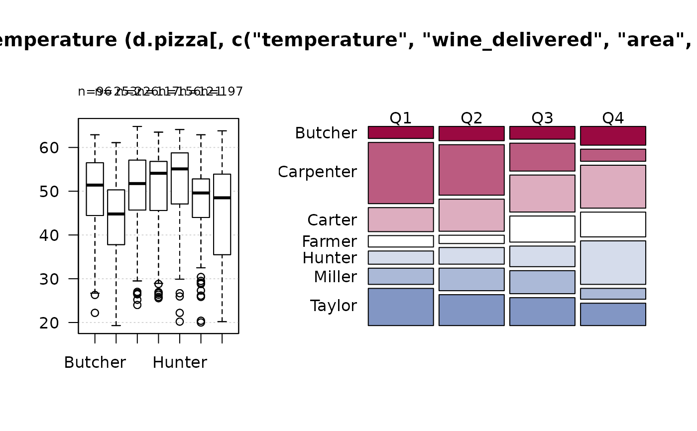 #> ──────────────────────────────────────────────────────────────────────────────
#> driver ~ area (d.pizza[, c("temperature", "wine_delivered", "area", "driver")])
#>
#> Summary:
#> n: 1'194, rows: 3, columns: 7
#>
#> Pearson's Chi-squared test:
#> X-squared = 1009.5, df = 12, p-value < 2.2e-16
#> Log likelihood ratio (G-test) test of independence:
#> G = 1020.9, X-squared df = 12, p-value < 2.2e-16
#> Mantel-Haenszel Chi-squared:
#> X-squared = 2.6144, df = 1, p-value = 0.1059
#>
#> Contingency Coeff. 0.677
#> Cramer's V 0.650
#> Kendall Tau-b -0.057
#>
#>
#> driver Butcher Carpenter Carter Farmer Hunter Miller
#> area
#>
#> Brent freq 72 29 177 19 128 6
#> perc 6.0% 2.4% 14.8% 1.6% 10.7% 0.5%
#> p.row 15.2% 6.1% 37.4% 4.0% 27.1% 1.3%
#> p.col 75.8% 10.8% 77.3% 16.2% 82.1% 4.8%
#>
#> Camden freq 1 19 47 87 4 41
#> perc 0.1% 1.6% 3.9% 7.3% 0.3% 3.4%
#> p.row 0.3% 5.6% 13.8% 25.5% 1.2% 12.0%
#> p.col 1.1% 7.1% 20.5% 74.4% 2.6% 33.1%
#>
#> Westminster freq 22 221 5 11 24 77
#> perc 1.8% 18.5% 0.4% 0.9% 2.0% 6.4%
#> p.row 5.8% 58.2% 1.3% 2.9% 6.3% 20.3%
#> p.col 23.2% 82.2% 2.2% 9.4% 15.4% 62.1%
#>
#> Sum freq 95 269 229 117 156 124
#> perc 8.0% 22.5% 19.2% 9.8% 13.1% 10.4%
#> p.row . . . . . .
#> p.col . . . . . .
#>
#>
#> driver Taylor Sum
#> area
#>
#> Brent freq 42 473
#> perc 3.5% 39.6%
#> p.row 8.9% .
#> p.col 20.6% .
#>
#> Camden freq 142 341
#> perc 11.9% 28.6%
#> p.row 41.6% .
#> p.col 69.6% .
#>
#> Westminster freq 20 380
#> perc 1.7% 31.8%
#> p.row 5.3% .
#> p.col 9.8% .
#>
#> Sum freq 204 1'194
#> perc 17.1% 100.0%
#> p.row . .
#> p.col . .
#>
#>
#> ──────────────────────────────────────────────────────────────────────────────
#> driver ~ area (d.pizza[, c("temperature", "wine_delivered", "area", "driver")])
#>
#> Summary:
#> n: 1'194, rows: 3, columns: 7
#>
#> Pearson's Chi-squared test:
#> X-squared = 1009.5, df = 12, p-value < 2.2e-16
#> Log likelihood ratio (G-test) test of independence:
#> G = 1020.9, X-squared df = 12, p-value < 2.2e-16
#> Mantel-Haenszel Chi-squared:
#> X-squared = 2.6144, df = 1, p-value = 0.1059
#>
#> Contingency Coeff. 0.677
#> Cramer's V 0.650
#> Kendall Tau-b -0.057
#>
#>
#> driver Butcher Carpenter Carter Farmer Hunter Miller
#> area
#>
#> Brent freq 72 29 177 19 128 6
#> perc 6.0% 2.4% 14.8% 1.6% 10.7% 0.5%
#> p.row 15.2% 6.1% 37.4% 4.0% 27.1% 1.3%
#> p.col 75.8% 10.8% 77.3% 16.2% 82.1% 4.8%
#>
#> Camden freq 1 19 47 87 4 41
#> perc 0.1% 1.6% 3.9% 7.3% 0.3% 3.4%
#> p.row 0.3% 5.6% 13.8% 25.5% 1.2% 12.0%
#> p.col 1.1% 7.1% 20.5% 74.4% 2.6% 33.1%
#>
#> Westminster freq 22 221 5 11 24 77
#> perc 1.8% 18.5% 0.4% 0.9% 2.0% 6.4%
#> p.row 5.8% 58.2% 1.3% 2.9% 6.3% 20.3%
#> p.col 23.2% 82.2% 2.2% 9.4% 15.4% 62.1%
#>
#> Sum freq 95 269 229 117 156 124
#> perc 8.0% 22.5% 19.2% 9.8% 13.1% 10.4%
#> p.row . . . . . .
#> p.col . . . . . .
#>
#>
#> driver Taylor Sum
#> area
#>
#> Brent freq 42 473
#> perc 3.5% 39.6%
#> p.row 8.9% .
#> p.col 20.6% .
#>
#> Camden freq 142 341
#> perc 11.9% 28.6%
#> p.row 41.6% .
#> p.col 69.6% .
#>
#> Westminster freq 20 380
#> perc 1.7% 31.8%
#> p.row 5.3% .
#> p.col 9.8% .
#>
#> Sum freq 204 1'194
#> perc 17.1% 100.0%
#> p.row . .
#> p.col . .
#>
#>
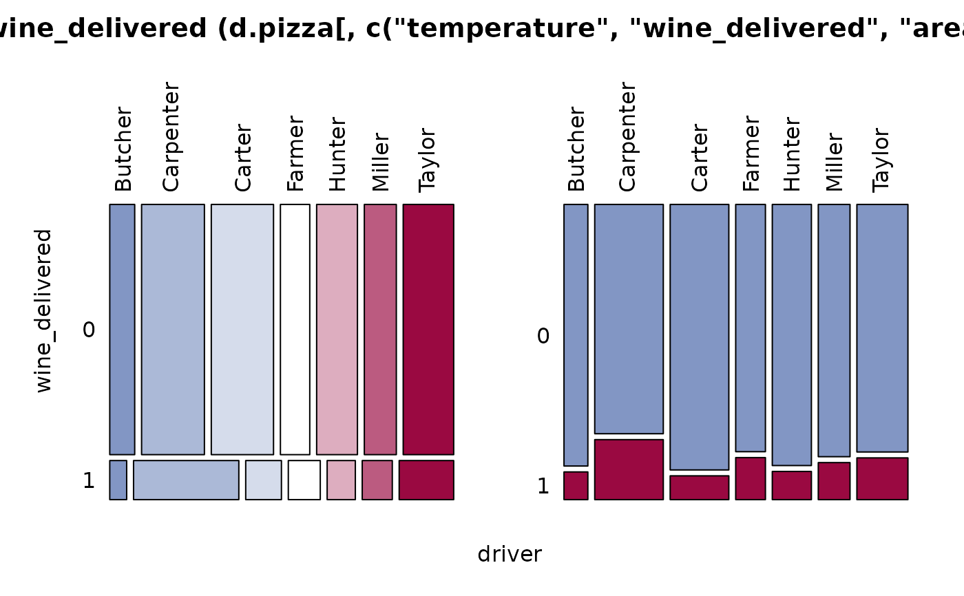 # all the rest versus response
Desc(. ~ driver, data=d.pizza[, c("temperature","wine_delivered","area","driver")])
#> ──────────────────────────────────────────────────────────────────────────────
#> temperature ~ driver (d.pizza[, c("temperature", "wine_delivered", "area", "driver")])
#>
#> Summary:
#> n pairs: 1'209, valid: 1'166 (96.4%), missings: 43 (3.6%), groups: 7
#>
#>
#> Butcher Carpenter Carter Farmer Hunter Miller
#> mean 49.61719 43.49348 50.41925 50.93675 52.14135 47.52397
#> median 51.40000 44.80000 51.75000 54.10000 55.10000 49.60000
#> sd 8.78704 9.40667 8.46700 9.02373 8.88544 8.93474
#> IQR 11.97500 12.50000 11.32500 11.20000 11.57500 8.80000
#> n 96 253 226 117 156 121
#> np 8.23328% 21.69811% 19.38250% 10.03431% 13.37907% 10.37736%
#> NAs 0 19 8 0 0 4
#> 0s 0 0 0 0 0 0
#>
#> Taylor
#> mean 45.09061
#> median 48.50000
#> sd 11.44201
#> IQR 18.40000
#> n 197
#> np 16.89537%
#> NAs 7
#> 0s 0
#>
#> Kruskal-Wallis rank sum test:
#> Kruskal-Wallis chi-squared = 141.93, df = 6, p-value < 2.2e-16
#>
#>
#> Warning:
#> Grouping variable contains 5 NAs (0.414%).
#>
# all the rest versus response
Desc(. ~ driver, data=d.pizza[, c("temperature","wine_delivered","area","driver")])
#> ──────────────────────────────────────────────────────────────────────────────
#> temperature ~ driver (d.pizza[, c("temperature", "wine_delivered", "area", "driver")])
#>
#> Summary:
#> n pairs: 1'209, valid: 1'166 (96.4%), missings: 43 (3.6%), groups: 7
#>
#>
#> Butcher Carpenter Carter Farmer Hunter Miller
#> mean 49.61719 43.49348 50.41925 50.93675 52.14135 47.52397
#> median 51.40000 44.80000 51.75000 54.10000 55.10000 49.60000
#> sd 8.78704 9.40667 8.46700 9.02373 8.88544 8.93474
#> IQR 11.97500 12.50000 11.32500 11.20000 11.57500 8.80000
#> n 96 253 226 117 156 121
#> np 8.23328% 21.69811% 19.38250% 10.03431% 13.37907% 10.37736%
#> NAs 0 19 8 0 0 4
#> 0s 0 0 0 0 0 0
#>
#> Taylor
#> mean 45.09061
#> median 48.50000
#> sd 11.44201
#> IQR 18.40000
#> n 197
#> np 16.89537%
#> NAs 7
#> 0s 0
#>
#> Kruskal-Wallis rank sum test:
#> Kruskal-Wallis chi-squared = 141.93, df = 6, p-value < 2.2e-16
#>
#>
#> Warning:
#> Grouping variable contains 5 NAs (0.414%).
#>
 #> ──────────────────────────────────────────────────────────────────────────────
#> wine_delivered ~ driver (d.pizza[, c("temperature", "wine_delivered", "area", "driver")])
#>
#> Summary:
#> n: 1'192, rows: 7, columns: 2
#>
#> Pearson's Chi-squared test:
#> X-squared = 21.029, df = 6, p-value = 0.001813
#> Log likelihood ratio (G-test) test of independence:
#> G = 20.646, X-squared df = 6, p-value = 0.002123
#> Mantel-Haenszel Chi-squared:
#> X-squared = 0.58591, df = 1, p-value = 0.444
#>
#> Contingency Coeff. 0.132
#> Cramer's V 0.133
#> Kendall Tau-b -0.026
#>
#>
#> wine_delivered 0 1 Sum
#> driver
#>
#> Butcher freq 85 9 94
#> perc 7.1% 0.8% 7.9%
#> p.row 90.4% 9.6% .
#> p.col 8.2% 5.6% .
#>
#> Carpenter freq 214 56 270
#> perc 18.0% 4.7% 22.7%
#> p.row 79.3% 20.7% .
#> p.col 20.8% 34.8% .
#>
#> Carter freq 212 19 231
#> perc 17.8% 1.6% 19.4%
#> p.row 91.8% 8.2% .
#> p.col 20.6% 11.8% .
#>
#> Farmer freq 100 17 117
#> perc 8.4% 1.4% 9.8%
#> p.row 85.5% 14.5% .
#> p.col 9.7% 10.6% .
#>
#> Hunter freq 139 15 154
#> perc 11.7% 1.3% 12.9%
#> p.row 90.3% 9.7% .
#> p.col 13.5% 9.3% .
#>
#> Miller freq 109 16 125
#> perc 9.1% 1.3% 10.5%
#> p.row 87.2% 12.8% .
#> p.col 10.6% 9.9% .
#>
#> Taylor freq 172 29 201
#> perc 14.4% 2.4% 16.9%
#> p.row 85.6% 14.4% .
#> p.col 16.7% 18.0% .
#>
#> Sum freq 1'031 161 1'192
#> perc 86.5% 13.5% 100.0%
#> p.row . . .
#> p.col . . .
#>
#>
#> ──────────────────────────────────────────────────────────────────────────────
#> wine_delivered ~ driver (d.pizza[, c("temperature", "wine_delivered", "area", "driver")])
#>
#> Summary:
#> n: 1'192, rows: 7, columns: 2
#>
#> Pearson's Chi-squared test:
#> X-squared = 21.029, df = 6, p-value = 0.001813
#> Log likelihood ratio (G-test) test of independence:
#> G = 20.646, X-squared df = 6, p-value = 0.002123
#> Mantel-Haenszel Chi-squared:
#> X-squared = 0.58591, df = 1, p-value = 0.444
#>
#> Contingency Coeff. 0.132
#> Cramer's V 0.133
#> Kendall Tau-b -0.026
#>
#>
#> wine_delivered 0 1 Sum
#> driver
#>
#> Butcher freq 85 9 94
#> perc 7.1% 0.8% 7.9%
#> p.row 90.4% 9.6% .
#> p.col 8.2% 5.6% .
#>
#> Carpenter freq 214 56 270
#> perc 18.0% 4.7% 22.7%
#> p.row 79.3% 20.7% .
#> p.col 20.8% 34.8% .
#>
#> Carter freq 212 19 231
#> perc 17.8% 1.6% 19.4%
#> p.row 91.8% 8.2% .
#> p.col 20.6% 11.8% .
#>
#> Farmer freq 100 17 117
#> perc 8.4% 1.4% 9.8%
#> p.row 85.5% 14.5% .
#> p.col 9.7% 10.6% .
#>
#> Hunter freq 139 15 154
#> perc 11.7% 1.3% 12.9%
#> p.row 90.3% 9.7% .
#> p.col 13.5% 9.3% .
#>
#> Miller freq 109 16 125
#> perc 9.1% 1.3% 10.5%
#> p.row 87.2% 12.8% .
#> p.col 10.6% 9.9% .
#>
#> Taylor freq 172 29 201
#> perc 14.4% 2.4% 16.9%
#> p.row 85.6% 14.4% .
#> p.col 16.7% 18.0% .
#>
#> Sum freq 1'031 161 1'192
#> perc 86.5% 13.5% 100.0%
#> p.row . . .
#> p.col . . .
#>
#>
 #> ──────────────────────────────────────────────────────────────────────────────
#> area ~ driver (d.pizza[, c("temperature", "wine_delivered", "area", "driver")])
#>
#> Summary:
#> n: 1'194, rows: 7, columns: 3
#>
#> Pearson's Chi-squared test:
#> X-squared = 1009.5, df = 12, p-value < 2.2e-16
#> Log likelihood ratio (G-test) test of independence:
#> G = 1020.9, X-squared df = 12, p-value < 2.2e-16
#> Mantel-Haenszel Chi-squared:
#> X-squared = 2.6144, df = 1, p-value = 0.1059
#>
#> Contingency Coeff. 0.677
#> Cramer's V 0.650
#> Kendall Tau-b -0.057
#>
#>
#> area Brent Camden Westminster Sum
#> driver
#>
#> Butcher freq 72 1 22 95
#> perc 6.0% 0.1% 1.8% 8.0%
#> p.row 75.8% 1.1% 23.2% .
#> p.col 15.2% 0.3% 5.8% .
#>
#> Carpenter freq 29 19 221 269
#> perc 2.4% 1.6% 18.5% 22.5%
#> p.row 10.8% 7.1% 82.2% .
#> p.col 6.1% 5.6% 58.2% .
#>
#> Carter freq 177 47 5 229
#> perc 14.8% 3.9% 0.4% 19.2%
#> p.row 77.3% 20.5% 2.2% .
#> p.col 37.4% 13.8% 1.3% .
#>
#> Farmer freq 19 87 11 117
#> perc 1.6% 7.3% 0.9% 9.8%
#> p.row 16.2% 74.4% 9.4% .
#> p.col 4.0% 25.5% 2.9% .
#>
#> Hunter freq 128 4 24 156
#> perc 10.7% 0.3% 2.0% 13.1%
#> p.row 82.1% 2.6% 15.4% .
#> p.col 27.1% 1.2% 6.3% .
#>
#> Miller freq 6 41 77 124
#> perc 0.5% 3.4% 6.4% 10.4%
#> p.row 4.8% 33.1% 62.1% .
#> p.col 1.3% 12.0% 20.3% .
#>
#> Taylor freq 42 142 20 204
#> perc 3.5% 11.9% 1.7% 17.1%
#> p.row 20.6% 69.6% 9.8% .
#> p.col 8.9% 41.6% 5.3% .
#>
#> Sum freq 473 341 380 1'194
#> perc 39.6% 28.6% 31.8% 100.0%
#> p.row . . . .
#> p.col . . . .
#>
#>
#> ──────────────────────────────────────────────────────────────────────────────
#> area ~ driver (d.pizza[, c("temperature", "wine_delivered", "area", "driver")])
#>
#> Summary:
#> n: 1'194, rows: 7, columns: 3
#>
#> Pearson's Chi-squared test:
#> X-squared = 1009.5, df = 12, p-value < 2.2e-16
#> Log likelihood ratio (G-test) test of independence:
#> G = 1020.9, X-squared df = 12, p-value < 2.2e-16
#> Mantel-Haenszel Chi-squared:
#> X-squared = 2.6144, df = 1, p-value = 0.1059
#>
#> Contingency Coeff. 0.677
#> Cramer's V 0.650
#> Kendall Tau-b -0.057
#>
#>
#> area Brent Camden Westminster Sum
#> driver
#>
#> Butcher freq 72 1 22 95
#> perc 6.0% 0.1% 1.8% 8.0%
#> p.row 75.8% 1.1% 23.2% .
#> p.col 15.2% 0.3% 5.8% .
#>
#> Carpenter freq 29 19 221 269
#> perc 2.4% 1.6% 18.5% 22.5%
#> p.row 10.8% 7.1% 82.2% .
#> p.col 6.1% 5.6% 58.2% .
#>
#> Carter freq 177 47 5 229
#> perc 14.8% 3.9% 0.4% 19.2%
#> p.row 77.3% 20.5% 2.2% .
#> p.col 37.4% 13.8% 1.3% .
#>
#> Farmer freq 19 87 11 117
#> perc 1.6% 7.3% 0.9% 9.8%
#> p.row 16.2% 74.4% 9.4% .
#> p.col 4.0% 25.5% 2.9% .
#>
#> Hunter freq 128 4 24 156
#> perc 10.7% 0.3% 2.0% 13.1%
#> p.row 82.1% 2.6% 15.4% .
#> p.col 27.1% 1.2% 6.3% .
#>
#> Miller freq 6 41 77 124
#> perc 0.5% 3.4% 6.4% 10.4%
#> p.row 4.8% 33.1% 62.1% .
#> p.col 1.3% 12.0% 20.3% .
#>
#> Taylor freq 42 142 20 204
#> perc 3.5% 11.9% 1.7% 17.1%
#> p.row 20.6% 69.6% 9.8% .
#> p.col 8.9% 41.6% 5.3% .
#>
#> Sum freq 473 341 380 1'194
#> perc 39.6% 28.6% 31.8% 100.0%
#> p.row . . . .
#> p.col . . . .
#>
#>
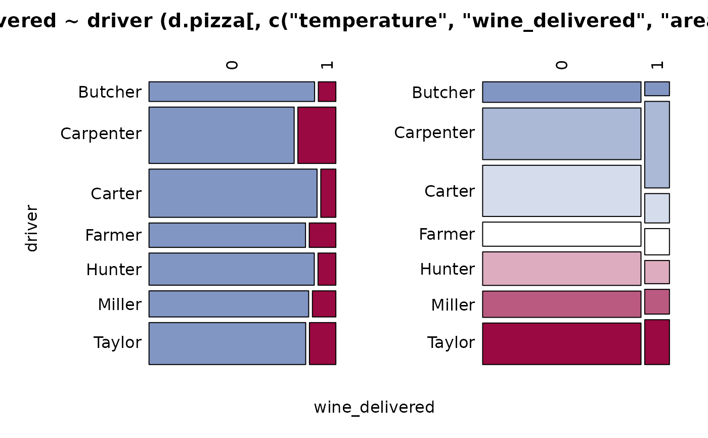 # pairwise Descriptions
p <- CombPairs(c("area","count","operator","driver","temperature","wrongpizza","quality"), )
for(i in 1:nrow(p))
print(Desc(formula(gettextf("%s ~ %s", p$X1[i], p$X2[i])), data=d.pizza))
#> ──────────────────────────────────────────────────────────────────────────────
#> area ~ count (d.pizza)
#>
#> Summary:
#> n pairs: 1'209, valid: 1'187 (98.2%), missings: 22 (1.8%), groups: 3
#>
#>
#> Brent Camden Westminster
#> mean 3.37045 3.40643 3.56614
#> median 3.00000 3.00000 3.00000
#> sd 1.54122 1.48946 1.62609
#> IQR 2.00000 2.00000 3.00000
#> n 467 342 378
#> np 39.34288% 28.81213% 31.84499%
#> NAs 7 2 3
#> 0s 0 0 0
#>
#> Kruskal-Wallis rank sum test:
#> Kruskal-Wallis chi-squared = 2.8703, df = 2, p-value = 0.2381
#>
#>
#> Warning:
#> Grouping variable contains 10 NAs (0.827%).
#>
#>
#>
#> Proportions of area in the quantiles of count:
#>
#> Q1 Q2 Q3 Q4
#> Brent 40.9% 39.9% 38.4% 37.5%
#> Camden 28.6% 30.9% 29.5% 26.4%
#> Westminster 30.5% 29.2% 32.1% 36.1%
#>
# pairwise Descriptions
p <- CombPairs(c("area","count","operator","driver","temperature","wrongpizza","quality"), )
for(i in 1:nrow(p))
print(Desc(formula(gettextf("%s ~ %s", p$X1[i], p$X2[i])), data=d.pizza))
#> ──────────────────────────────────────────────────────────────────────────────
#> area ~ count (d.pizza)
#>
#> Summary:
#> n pairs: 1'209, valid: 1'187 (98.2%), missings: 22 (1.8%), groups: 3
#>
#>
#> Brent Camden Westminster
#> mean 3.37045 3.40643 3.56614
#> median 3.00000 3.00000 3.00000
#> sd 1.54122 1.48946 1.62609
#> IQR 2.00000 2.00000 3.00000
#> n 467 342 378
#> np 39.34288% 28.81213% 31.84499%
#> NAs 7 2 3
#> 0s 0 0 0
#>
#> Kruskal-Wallis rank sum test:
#> Kruskal-Wallis chi-squared = 2.8703, df = 2, p-value = 0.2381
#>
#>
#> Warning:
#> Grouping variable contains 10 NAs (0.827%).
#>
#>
#>
#> Proportions of area in the quantiles of count:
#>
#> Q1 Q2 Q3 Q4
#> Brent 40.9% 39.9% 38.4% 37.5%
#> Camden 28.6% 30.9% 29.5% 26.4%
#> Westminster 30.5% 29.2% 32.1% 36.1%
#>
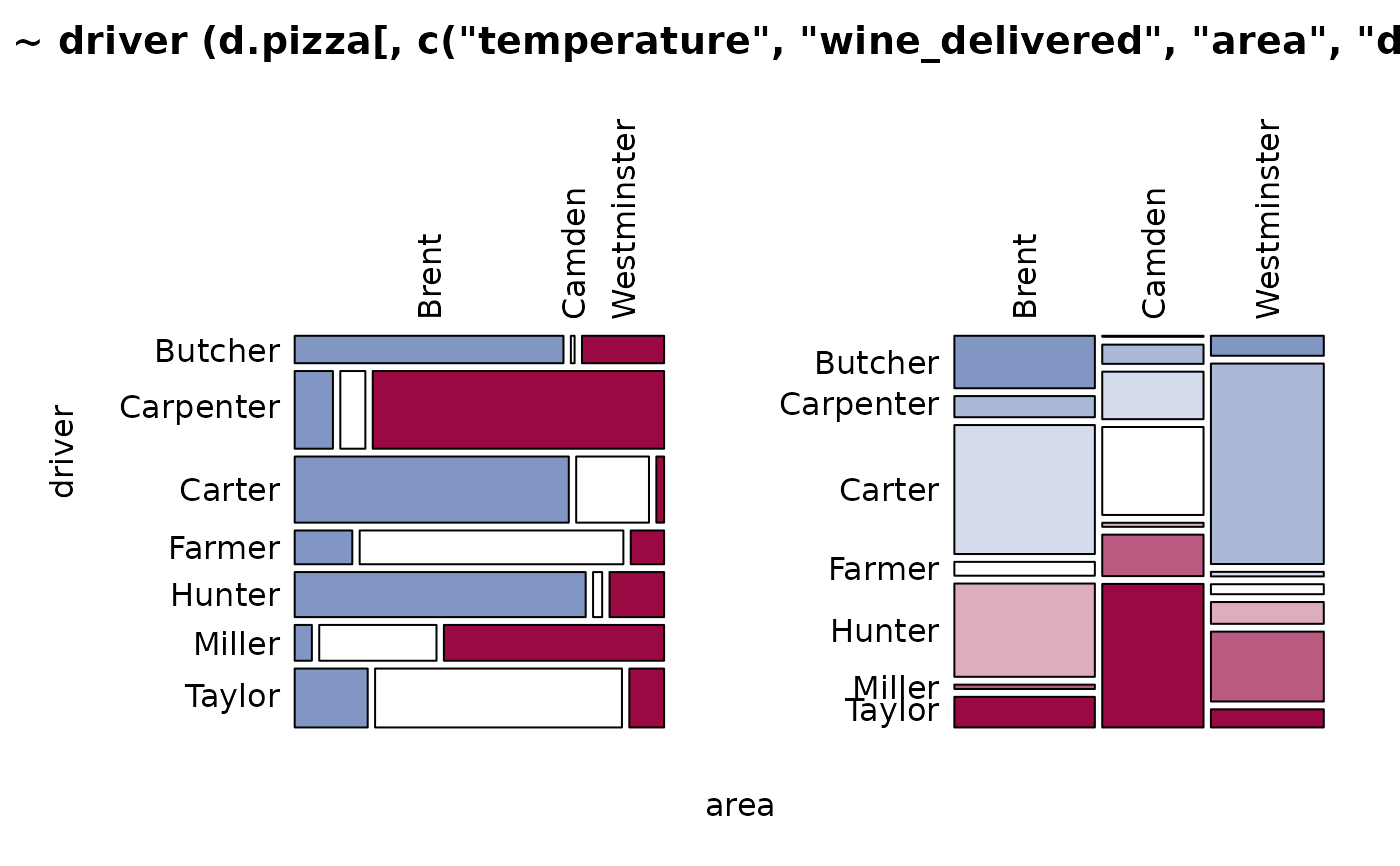 #> Warning: argument 1 does not name a graphical parameter
#> ──────────────────────────────────────────────────────────────────────────────
#> area ~ operator (d.pizza)
#>
#> Summary:
#> n: 1'191, rows: 3, columns: 3
#>
#> Pearson's Chi-squared test:
#> X-squared = 17.905, df = 4, p-value = 0.001288
#> Log likelihood ratio (G-test) test of independence:
#> G = 18.099, X-squared df = 4, p-value = 0.001181
#> Mantel-Haenszel Chi-squared:
#> X-squared = 8.6654, df = 1, p-value = 0.003243
#>
#> Contingency Coeff. 0.122
#> Cramer's V 0.087
#> Kendall Tau-b 0.073
#>
#>
#> area Brent Camden Westminster Sum
#> operator
#>
#> Allanah freq 153 123 89 365
#> perc 12.8% 10.3% 7.5% 30.6%
#> p.row 41.9% 33.7% 24.4% .
#> p.col 32.3% 36.2% 23.5% .
#>
#> Maria freq 153 108 122 383
#> perc 12.8% 9.1% 10.2% 32.2%
#> p.row 39.9% 28.2% 31.9% .
#> p.col 32.3% 31.8% 32.3% .
#>
#> Rhonda freq 167 109 167 443
#> perc 14.0% 9.2% 14.0% 37.2%
#> p.row 37.7% 24.6% 37.7% .
#> p.col 35.3% 32.1% 44.2% .
#>
#> Sum freq 473 340 378 1'191
#> perc 39.7% 28.5% 31.7% 100.0%
#> p.row . . . .
#> p.col . . . .
#>
#>
#> Warning: argument 1 does not name a graphical parameter
#> ──────────────────────────────────────────────────────────────────────────────
#> area ~ operator (d.pizza)
#>
#> Summary:
#> n: 1'191, rows: 3, columns: 3
#>
#> Pearson's Chi-squared test:
#> X-squared = 17.905, df = 4, p-value = 0.001288
#> Log likelihood ratio (G-test) test of independence:
#> G = 18.099, X-squared df = 4, p-value = 0.001181
#> Mantel-Haenszel Chi-squared:
#> X-squared = 8.6654, df = 1, p-value = 0.003243
#>
#> Contingency Coeff. 0.122
#> Cramer's V 0.087
#> Kendall Tau-b 0.073
#>
#>
#> area Brent Camden Westminster Sum
#> operator
#>
#> Allanah freq 153 123 89 365
#> perc 12.8% 10.3% 7.5% 30.6%
#> p.row 41.9% 33.7% 24.4% .
#> p.col 32.3% 36.2% 23.5% .
#>
#> Maria freq 153 108 122 383
#> perc 12.8% 9.1% 10.2% 32.2%
#> p.row 39.9% 28.2% 31.9% .
#> p.col 32.3% 31.8% 32.3% .
#>
#> Rhonda freq 167 109 167 443
#> perc 14.0% 9.2% 14.0% 37.2%
#> p.row 37.7% 24.6% 37.7% .
#> p.col 35.3% 32.1% 44.2% .
#>
#> Sum freq 473 340 378 1'191
#> perc 39.7% 28.5% 31.7% 100.0%
#> p.row . . . .
#> p.col . . . .
#>
#>
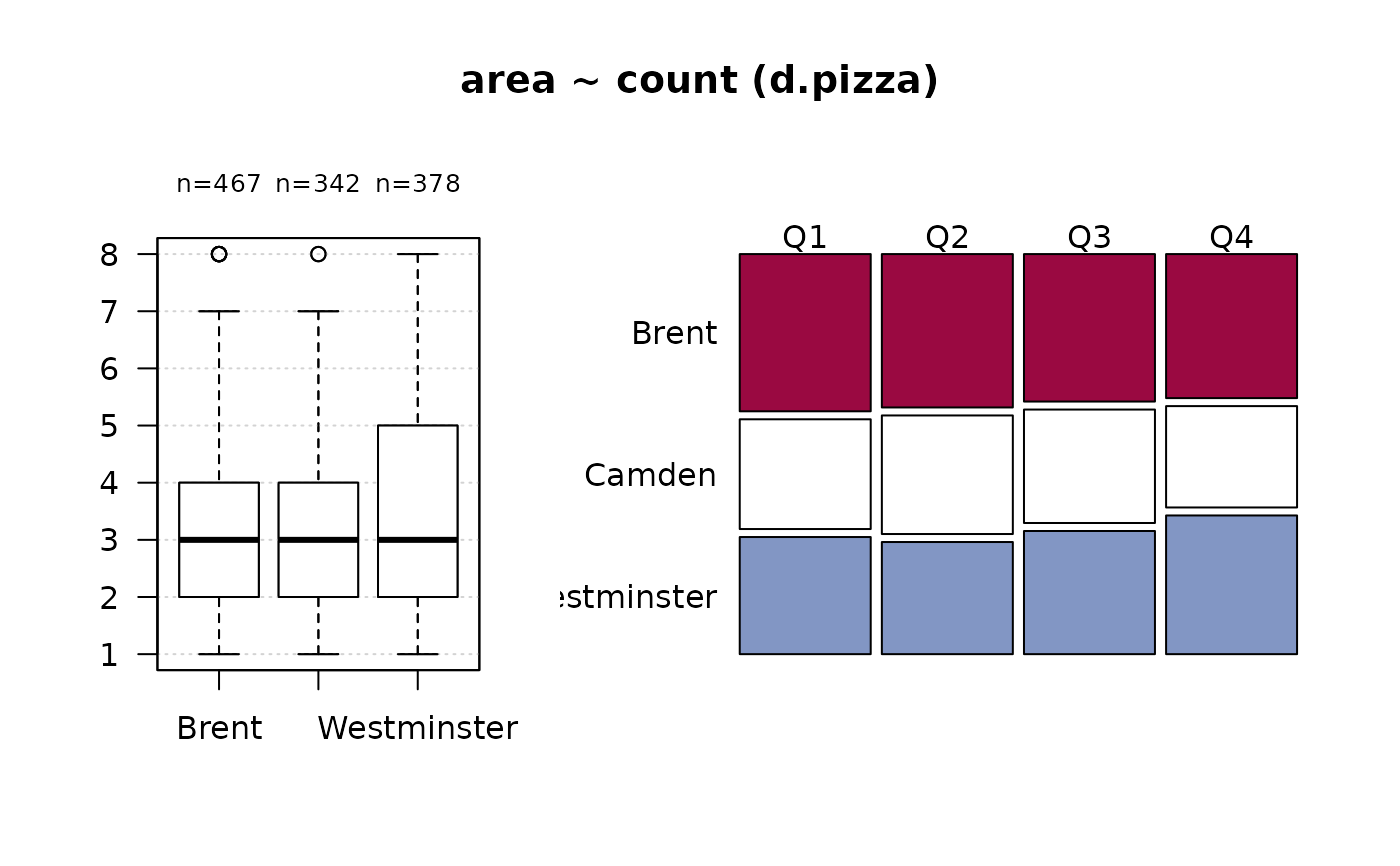 #> ──────────────────────────────────────────────────────────────────────────────
#> area ~ driver (d.pizza)
#>
#> Summary:
#> n: 1'194, rows: 7, columns: 3
#>
#> Pearson's Chi-squared test:
#> X-squared = 1009.5, df = 12, p-value < 2.2e-16
#> Log likelihood ratio (G-test) test of independence:
#> G = 1020.9, X-squared df = 12, p-value < 2.2e-16
#> Mantel-Haenszel Chi-squared:
#> X-squared = 2.6144, df = 1, p-value = 0.1059
#>
#> Contingency Coeff. 0.677
#> Cramer's V 0.650
#> Kendall Tau-b -0.057
#>
#>
#> area Brent Camden Westminster Sum
#> driver
#>
#> Butcher freq 72 1 22 95
#> perc 6.0% 0.1% 1.8% 8.0%
#> p.row 75.8% 1.1% 23.2% .
#> p.col 15.2% 0.3% 5.8% .
#>
#> Carpenter freq 29 19 221 269
#> perc 2.4% 1.6% 18.5% 22.5%
#> p.row 10.8% 7.1% 82.2% .
#> p.col 6.1% 5.6% 58.2% .
#>
#> Carter freq 177 47 5 229
#> perc 14.8% 3.9% 0.4% 19.2%
#> p.row 77.3% 20.5% 2.2% .
#> p.col 37.4% 13.8% 1.3% .
#>
#> Farmer freq 19 87 11 117
#> perc 1.6% 7.3% 0.9% 9.8%
#> p.row 16.2% 74.4% 9.4% .
#> p.col 4.0% 25.5% 2.9% .
#>
#> Hunter freq 128 4 24 156
#> perc 10.7% 0.3% 2.0% 13.1%
#> p.row 82.1% 2.6% 15.4% .
#> p.col 27.1% 1.2% 6.3% .
#>
#> Miller freq 6 41 77 124
#> perc 0.5% 3.4% 6.4% 10.4%
#> p.row 4.8% 33.1% 62.1% .
#> p.col 1.3% 12.0% 20.3% .
#>
#> Taylor freq 42 142 20 204
#> perc 3.5% 11.9% 1.7% 17.1%
#> p.row 20.6% 69.6% 9.8% .
#> p.col 8.9% 41.6% 5.3% .
#>
#> Sum freq 473 341 380 1'194
#> perc 39.6% 28.6% 31.8% 100.0%
#> p.row . . . .
#> p.col . . . .
#>
#>
#> ──────────────────────────────────────────────────────────────────────────────
#> area ~ driver (d.pizza)
#>
#> Summary:
#> n: 1'194, rows: 7, columns: 3
#>
#> Pearson's Chi-squared test:
#> X-squared = 1009.5, df = 12, p-value < 2.2e-16
#> Log likelihood ratio (G-test) test of independence:
#> G = 1020.9, X-squared df = 12, p-value < 2.2e-16
#> Mantel-Haenszel Chi-squared:
#> X-squared = 2.6144, df = 1, p-value = 0.1059
#>
#> Contingency Coeff. 0.677
#> Cramer's V 0.650
#> Kendall Tau-b -0.057
#>
#>
#> area Brent Camden Westminster Sum
#> driver
#>
#> Butcher freq 72 1 22 95
#> perc 6.0% 0.1% 1.8% 8.0%
#> p.row 75.8% 1.1% 23.2% .
#> p.col 15.2% 0.3% 5.8% .
#>
#> Carpenter freq 29 19 221 269
#> perc 2.4% 1.6% 18.5% 22.5%
#> p.row 10.8% 7.1% 82.2% .
#> p.col 6.1% 5.6% 58.2% .
#>
#> Carter freq 177 47 5 229
#> perc 14.8% 3.9% 0.4% 19.2%
#> p.row 77.3% 20.5% 2.2% .
#> p.col 37.4% 13.8% 1.3% .
#>
#> Farmer freq 19 87 11 117
#> perc 1.6% 7.3% 0.9% 9.8%
#> p.row 16.2% 74.4% 9.4% .
#> p.col 4.0% 25.5% 2.9% .
#>
#> Hunter freq 128 4 24 156
#> perc 10.7% 0.3% 2.0% 13.1%
#> p.row 82.1% 2.6% 15.4% .
#> p.col 27.1% 1.2% 6.3% .
#>
#> Miller freq 6 41 77 124
#> perc 0.5% 3.4% 6.4% 10.4%
#> p.row 4.8% 33.1% 62.1% .
#> p.col 1.3% 12.0% 20.3% .
#>
#> Taylor freq 42 142 20 204
#> perc 3.5% 11.9% 1.7% 17.1%
#> p.row 20.6% 69.6% 9.8% .
#> p.col 8.9% 41.6% 5.3% .
#>
#> Sum freq 473 341 380 1'194
#> perc 39.6% 28.6% 31.8% 100.0%
#> p.row . . . .
#> p.col . . . .
#>
#>
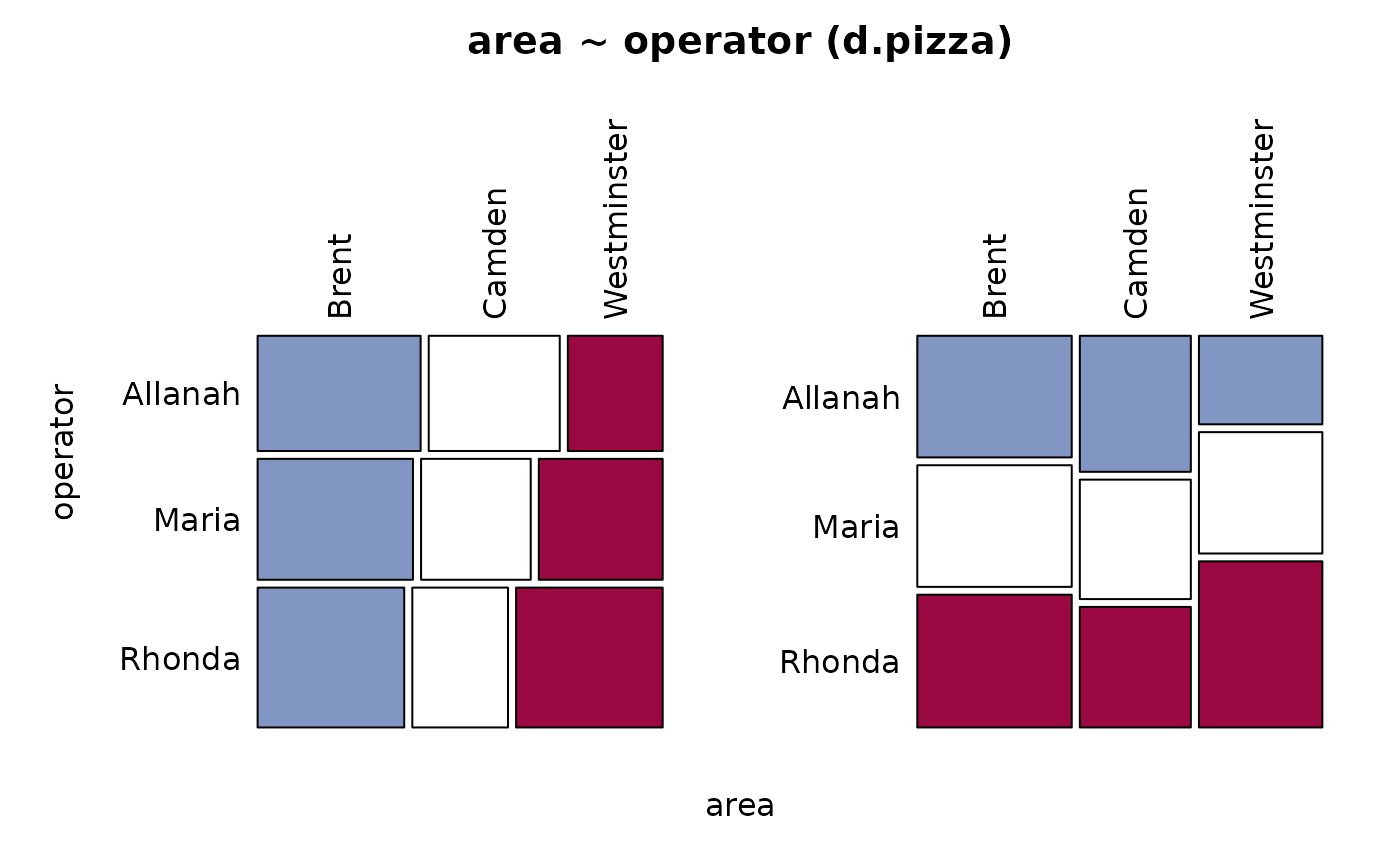 #> ──────────────────────────────────────────────────────────────────────────────
#> area ~ temperature (d.pizza)
#>
#> Summary:
#> n pairs: 1'209, valid: 1'161 (96.0%), missings: 48 (4.0%), groups: 3
#>
#>
#> Brent Camden Westminster
#> mean 51.13876 47.42030 44.25850
#> median 53.40000 50.30000 45.90000
#> sd 8.73353 10.11051 9.83558
#> IQR 10.50000 12.20000 13.20000
#> n 467 335 359
#> np 40.22394% 28.85444% 30.92162%
#> NAs 7 9 22
#> 0s 0 0 0
#>
#> Kruskal-Wallis rank sum test:
#> Kruskal-Wallis chi-squared = 115.83, df = 2, p-value < 2.2e-16
#>
#>
#> Warning:
#> Grouping variable contains 10 NAs (0.827%).
#>
#>
#>
#> Proportions of area in the quantiles of temperature:
#>
#> Q1 Q2 Q3 Q4
#> Brent 24.4% 34.5% 40.5% 61.8%
#> Camden 28.9% 26.6% 36.3% 23.6%
#> Westminster 46.7% 38.9% 23.2% 14.6%
#>
#> ──────────────────────────────────────────────────────────────────────────────
#> area ~ temperature (d.pizza)
#>
#> Summary:
#> n pairs: 1'209, valid: 1'161 (96.0%), missings: 48 (4.0%), groups: 3
#>
#>
#> Brent Camden Westminster
#> mean 51.13876 47.42030 44.25850
#> median 53.40000 50.30000 45.90000
#> sd 8.73353 10.11051 9.83558
#> IQR 10.50000 12.20000 13.20000
#> n 467 335 359
#> np 40.22394% 28.85444% 30.92162%
#> NAs 7 9 22
#> 0s 0 0 0
#>
#> Kruskal-Wallis rank sum test:
#> Kruskal-Wallis chi-squared = 115.83, df = 2, p-value < 2.2e-16
#>
#>
#> Warning:
#> Grouping variable contains 10 NAs (0.827%).
#>
#>
#>
#> Proportions of area in the quantiles of temperature:
#>
#> Q1 Q2 Q3 Q4
#> Brent 24.4% 34.5% 40.5% 61.8%
#> Camden 28.9% 26.6% 36.3% 23.6%
#> Westminster 46.7% 38.9% 23.2% 14.6%
#>
 #> Warning: argument 1 does not name a graphical parameter
#> ──────────────────────────────────────────────────────────────────────────────
#> area ~ wrongpizza (d.pizza)
#>
#> Summary:
#> n: 1'195, rows: 2, columns: 3
#>
#> Pearson's Chi-squared test:
#> X-squared = 1.3919, df = 2, p-value = 0.4986
#> Log likelihood ratio (G-test) test of independence:
#> G = 1.3558, X-squared df = 2, p-value = 0.5077
#> Mantel-Haenszel Chi-squared:
#> X-squared = 0.11732, df = 1, p-value = 0.732
#>
#> Contingency Coeff. 0.034
#> Cramer's V 0.034
#> Kendall Tau-b 0.010
#>
#>
#> area Brent Camden Westminster Sum
#> wrongpizza
#>
#> FALSE freq 445 314 354 1'113
#> perc 37.2% 26.3% 29.6% 93.1%
#> p.row 40.0% 28.2% 31.8% .
#> p.col 93.9% 91.8% 93.4% .
#>
#> TRUE freq 29 28 25 82
#> perc 2.4% 2.3% 2.1% 6.9%
#> p.row 35.4% 34.1% 30.5% .
#> p.col 6.1% 8.2% 6.6% .
#>
#> Sum freq 474 342 379 1'195
#> perc 39.7% 28.6% 31.7% 100.0%
#> p.row . . . .
#> p.col . . . .
#>
#>
#> Warning: argument 1 does not name a graphical parameter
#> ──────────────────────────────────────────────────────────────────────────────
#> area ~ wrongpizza (d.pizza)
#>
#> Summary:
#> n: 1'195, rows: 2, columns: 3
#>
#> Pearson's Chi-squared test:
#> X-squared = 1.3919, df = 2, p-value = 0.4986
#> Log likelihood ratio (G-test) test of independence:
#> G = 1.3558, X-squared df = 2, p-value = 0.5077
#> Mantel-Haenszel Chi-squared:
#> X-squared = 0.11732, df = 1, p-value = 0.732
#>
#> Contingency Coeff. 0.034
#> Cramer's V 0.034
#> Kendall Tau-b 0.010
#>
#>
#> area Brent Camden Westminster Sum
#> wrongpizza
#>
#> FALSE freq 445 314 354 1'113
#> perc 37.2% 26.3% 29.6% 93.1%
#> p.row 40.0% 28.2% 31.8% .
#> p.col 93.9% 91.8% 93.4% .
#>
#> TRUE freq 29 28 25 82
#> perc 2.4% 2.3% 2.1% 6.9%
#> p.row 35.4% 34.1% 30.5% .
#> p.col 6.1% 8.2% 6.6% .
#>
#> Sum freq 474 342 379 1'195
#> perc 39.7% 28.6% 31.7% 100.0%
#> p.row . . . .
#> p.col . . . .
#>
#>
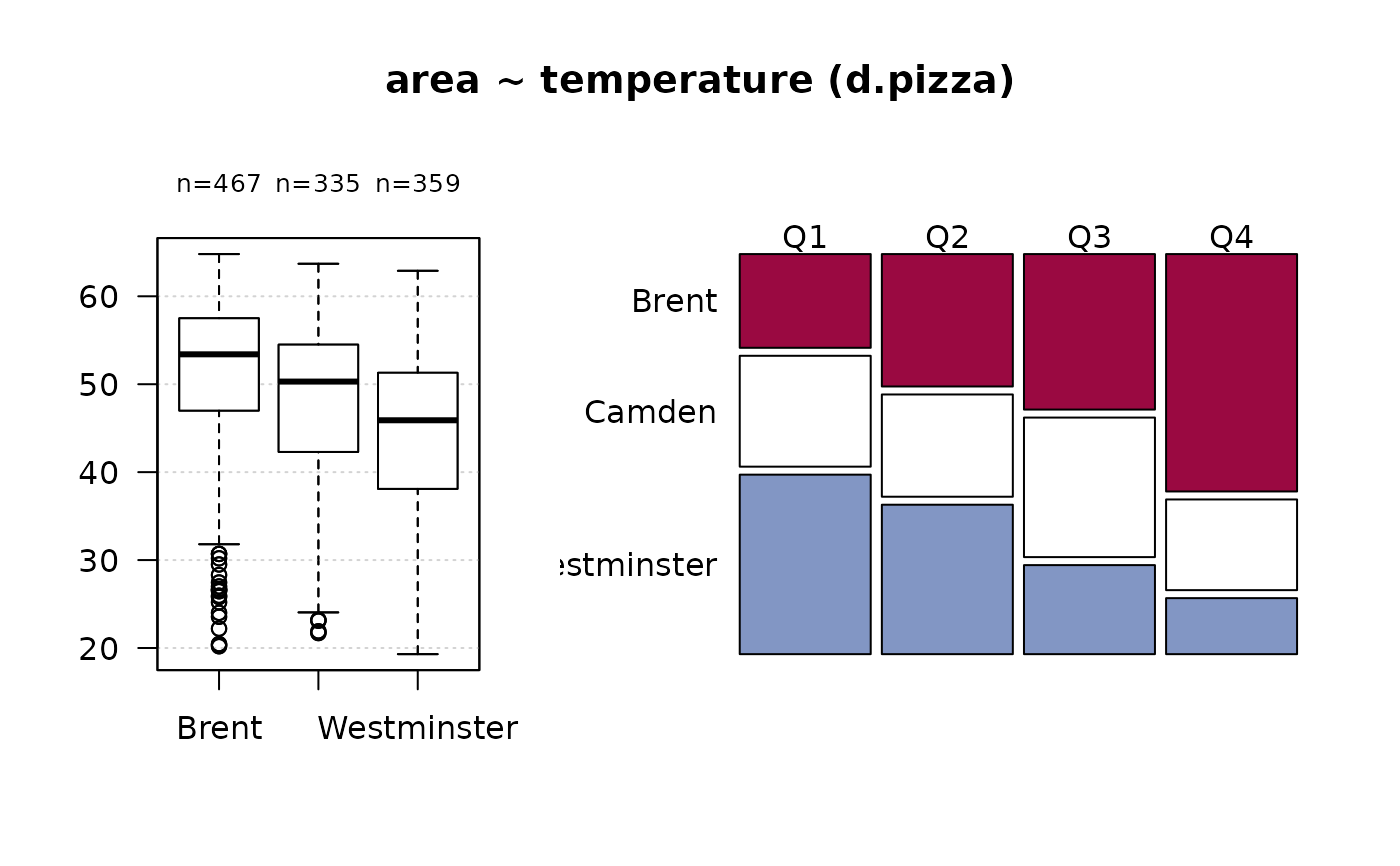 #> ──────────────────────────────────────────────────────────────────────────────
#> area ~ quality (d.pizza)
#>
#> Summary:
#> n: 999, rows: 3, columns: 3
#>
#> Pearson's Chi-squared test:
#> X-squared = 53.559, df = 4, p-value = 0.00000000006509
#> Log likelihood ratio (G-test) test of independence:
#> G = 55.05, X-squared df = 4, p-value = 0.00000000003171
#> Mantel-Haenszel Chi-squared:
#> X-squared = 51.341, df = 1, p-value = 7.762e-13
#>
#> Contingency Coeff. 0.226
#> Cramer's V 0.164
#> Kendall Tau-b -0.196
#>
#>
#> area Brent Camden Westminster Sum
#> quality
#>
#> low freq 30 46 79 155
#> perc 3.0% 4.6% 7.9% 15.5%
#> p.row 19.4% 29.7% 51.0% .
#> p.col 7.6% 16.0% 25.0% .
#>
#> medium freq 134 97 122 353
#> perc 13.4% 9.7% 12.2% 35.3%
#> p.row 38.0% 27.5% 34.6% .
#> p.col 33.8% 33.8% 38.6% .
#>
#> high freq 232 144 115 491
#> perc 23.2% 14.4% 11.5% 49.1%
#> p.row 47.3% 29.3% 23.4% .
#> p.col 58.6% 50.2% 36.4% .
#>
#> Sum freq 396 287 316 999
#> perc 39.6% 28.7% 31.6% 100.0%
#> p.row . . . .
#> p.col . . . .
#>
#>
#> ──────────────────────────────────────────────────────────────────────────────
#> area ~ quality (d.pizza)
#>
#> Summary:
#> n: 999, rows: 3, columns: 3
#>
#> Pearson's Chi-squared test:
#> X-squared = 53.559, df = 4, p-value = 0.00000000006509
#> Log likelihood ratio (G-test) test of independence:
#> G = 55.05, X-squared df = 4, p-value = 0.00000000003171
#> Mantel-Haenszel Chi-squared:
#> X-squared = 51.341, df = 1, p-value = 7.762e-13
#>
#> Contingency Coeff. 0.226
#> Cramer's V 0.164
#> Kendall Tau-b -0.196
#>
#>
#> area Brent Camden Westminster Sum
#> quality
#>
#> low freq 30 46 79 155
#> perc 3.0% 4.6% 7.9% 15.5%
#> p.row 19.4% 29.7% 51.0% .
#> p.col 7.6% 16.0% 25.0% .
#>
#> medium freq 134 97 122 353
#> perc 13.4% 9.7% 12.2% 35.3%
#> p.row 38.0% 27.5% 34.6% .
#> p.col 33.8% 33.8% 38.6% .
#>
#> high freq 232 144 115 491
#> perc 23.2% 14.4% 11.5% 49.1%
#> p.row 47.3% 29.3% 23.4% .
#> p.col 58.6% 50.2% 36.4% .
#>
#> Sum freq 396 287 316 999
#> perc 39.6% 28.7% 31.6% 100.0%
#> p.row . . . .
#> p.col . . . .
#>
#>
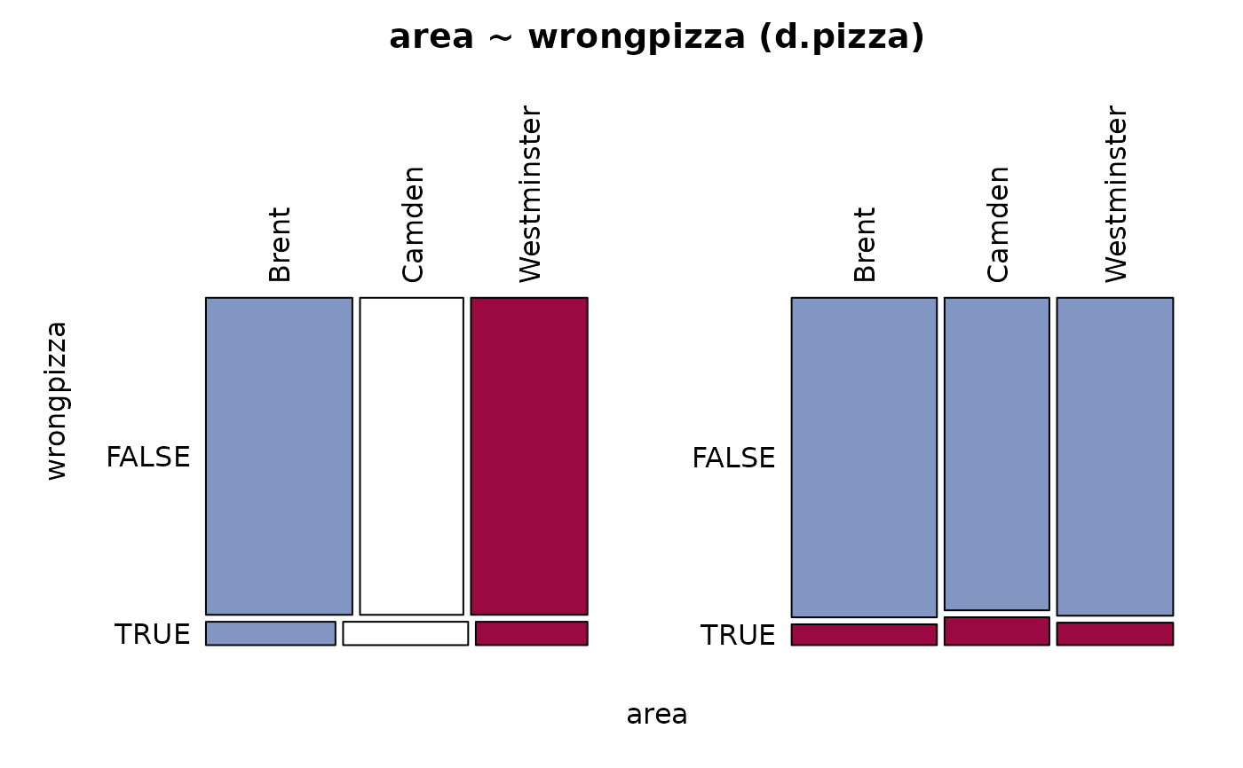 #> ──────────────────────────────────────────────────────────────────────────────
#> count ~ operator (d.pizza)
#>
#> Summary:
#> n pairs: 1'209, valid: 1'189 (98.3%), missings: 20 (1.7%), groups: 3
#>
#>
#> Allanah Maria Rhonda
#> mean 3.31129 3.53906 3.46154
#> median 3.00000 3.00000 3.00000
#> sd 1.45259 1.61537 1.57923
#> IQR 2.00000 3.00000 3.00000
#> n 363 384 442
#> np 30.52986% 32.29605% 37.17410%
#> NAs 4 4 4
#> 0s 0 0 0
#>
#> Kruskal-Wallis rank sum test:
#> Kruskal-Wallis chi-squared = 2.9148, df = 2, p-value = 0.2328
#>
#>
#> Warning:
#> Grouping variable contains 8 NAs (0.662%).
#>
#> ──────────────────────────────────────────────────────────────────────────────
#> count ~ operator (d.pizza)
#>
#> Summary:
#> n pairs: 1'209, valid: 1'189 (98.3%), missings: 20 (1.7%), groups: 3
#>
#>
#> Allanah Maria Rhonda
#> mean 3.31129 3.53906 3.46154
#> median 3.00000 3.00000 3.00000
#> sd 1.45259 1.61537 1.57923
#> IQR 2.00000 3.00000 3.00000
#> n 363 384 442
#> np 30.52986% 32.29605% 37.17410%
#> NAs 4 4 4
#> 0s 0 0 0
#>
#> Kruskal-Wallis rank sum test:
#> Kruskal-Wallis chi-squared = 2.9148, df = 2, p-value = 0.2328
#>
#>
#> Warning:
#> Grouping variable contains 8 NAs (0.662%).
#>
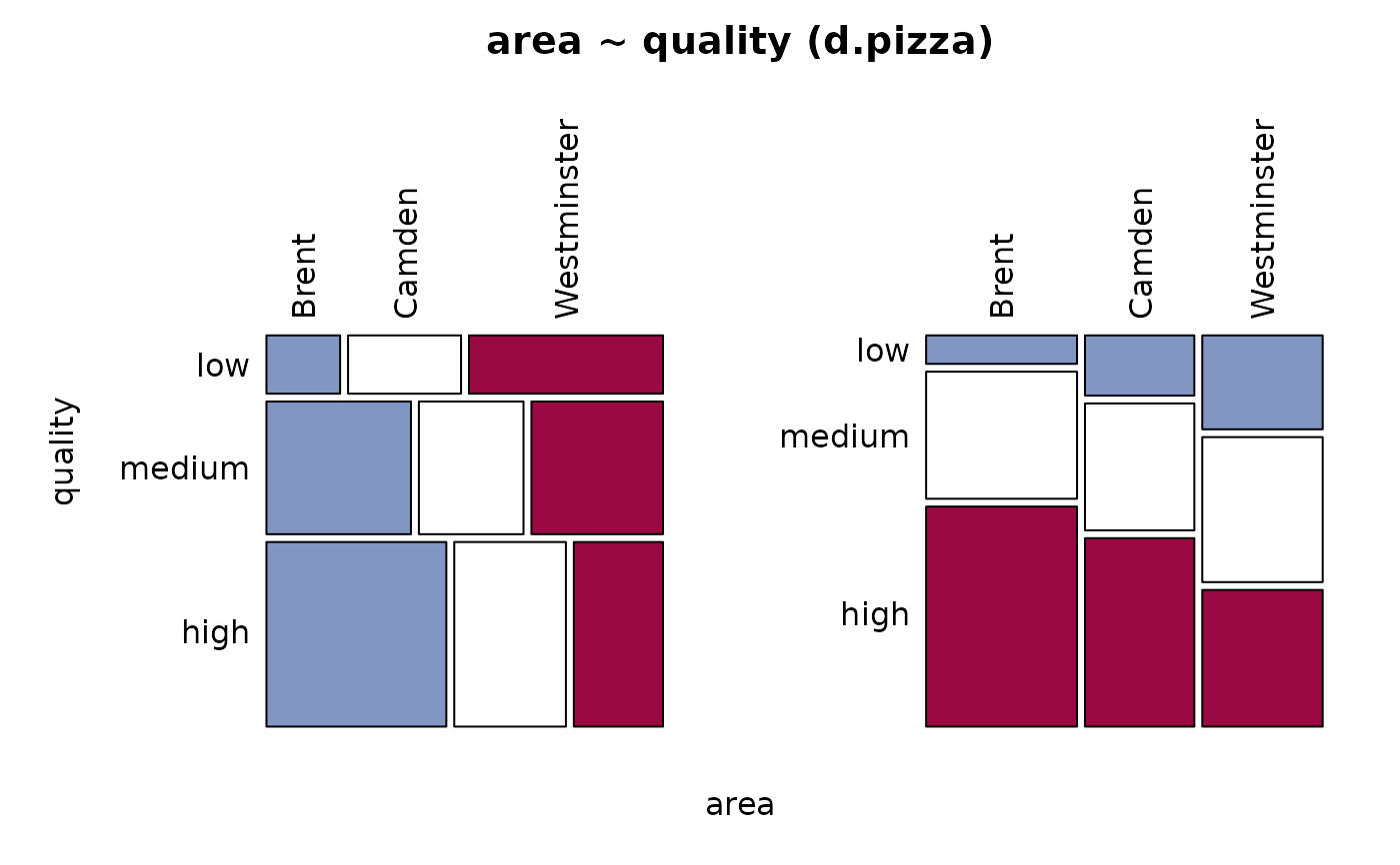 #> ──────────────────────────────────────────────────────────────────────────────
#> count ~ driver (d.pizza)
#>
#> Summary:
#> n pairs: 1'209, valid: 1'192 (98.6%), missings: 17 (1.4%), groups: 7
#>
#>
#> Butcher Carpenter Carter Farmer Hunter Miller
#> mean 3.25532 3.59259 3.40693 3.47863 3.28571 3.50400
#> median 3.00000 3.00000 3.00000 3.00000 3.00000 3.00000
#> sd 1.48784 1.58664 1.68336 1.39332 1.50257 1.67344
#> IQR 2.00000 3.00000 3.00000 1.00000 2.00000 2.00000
#> n 94 270 231 117 154 125
#> np 7.88591% 22.65101% 19.37919% 9.81544% 12.91946% 10.48658%
#> NAs 2 2 3 0 2 0
#> 0s 0 0 0 0 0 0
#>
#> Taylor
#> mean 3.45274
#> median 3.00000
#> sd 1.45568
#> IQR 2.00000
#> n 201
#> np 16.86242%
#> NAs 3
#> 0s 0
#>
#> Kruskal-Wallis rank sum test:
#> Kruskal-Wallis chi-squared = 5.5479, df = 6, p-value = 0.4757
#>
#>
#> Warning:
#> Grouping variable contains 5 NAs (0.414%).
#>
#> ──────────────────────────────────────────────────────────────────────────────
#> count ~ driver (d.pizza)
#>
#> Summary:
#> n pairs: 1'209, valid: 1'192 (98.6%), missings: 17 (1.4%), groups: 7
#>
#>
#> Butcher Carpenter Carter Farmer Hunter Miller
#> mean 3.25532 3.59259 3.40693 3.47863 3.28571 3.50400
#> median 3.00000 3.00000 3.00000 3.00000 3.00000 3.00000
#> sd 1.48784 1.58664 1.68336 1.39332 1.50257 1.67344
#> IQR 2.00000 3.00000 3.00000 1.00000 2.00000 2.00000
#> n 94 270 231 117 154 125
#> np 7.88591% 22.65101% 19.37919% 9.81544% 12.91946% 10.48658%
#> NAs 2 2 3 0 2 0
#> 0s 0 0 0 0 0 0
#>
#> Taylor
#> mean 3.45274
#> median 3.00000
#> sd 1.45568
#> IQR 2.00000
#> n 201
#> np 16.86242%
#> NAs 3
#> 0s 0
#>
#> Kruskal-Wallis rank sum test:
#> Kruskal-Wallis chi-squared = 5.5479, df = 6, p-value = 0.4757
#>
#>
#> Warning:
#> Grouping variable contains 5 NAs (0.414%).
#>
 #> ──────────────────────────────────────────────────────────────────────────────
#> count ~ temperature (d.pizza)
#>
#> Summary:
#> n pairs: 1'209, valid: 1'158 (95.8%), missings: 51 (4.2%)
#>
#>
#> Pearson corr. : 0.043
#> Spearman corr.: 0.030
#> Kendall corr. : 0.022
#>
#> ──────────────────────────────────────────────────────────────────────────────
#> count ~ temperature (d.pizza)
#>
#> Summary:
#> n pairs: 1'209, valid: 1'158 (95.8%), missings: 51 (4.2%)
#>
#>
#> Pearson corr. : 0.043
#> Spearman corr.: 0.030
#> Kendall corr. : 0.022
#>
 #> ──────────────────────────────────────────────────────────────────────────────
#> count ~ wrongpizza (d.pizza)
#>
#> Summary:
#> n pairs: 1'209, valid: 1'193 (98.7%), missings: 16 (1.3%), groups: 2
#>
#>
#> FALSE TRUE
#> mean 3.42934 3.68293
#> median 3.00000 3.00000
#> sd 1.53875 1.76997
#> IQR 2.00000 3.00000
#> n 1'111 82
#> np 93.12657% 6.87343%
#> NAs 11 1
#> 0s 0 0
#>
#> Kruskal-Wallis rank sum test:
#> Kruskal-Wallis chi-squared = 0.98439, df = 1, p-value = 0.3211
#>
#>
#> Warning:
#> Grouping variable contains 4 NAs (0.331%).
#>
#> ──────────────────────────────────────────────────────────────────────────────
#> count ~ wrongpizza (d.pizza)
#>
#> Summary:
#> n pairs: 1'209, valid: 1'193 (98.7%), missings: 16 (1.3%), groups: 2
#>
#>
#> FALSE TRUE
#> mean 3.42934 3.68293
#> median 3.00000 3.00000
#> sd 1.53875 1.76997
#> IQR 2.00000 3.00000
#> n 1'111 82
#> np 93.12657% 6.87343%
#> NAs 11 1
#> 0s 0 0
#>
#> Kruskal-Wallis rank sum test:
#> Kruskal-Wallis chi-squared = 0.98439, df = 1, p-value = 0.3211
#>
#>
#> Warning:
#> Grouping variable contains 4 NAs (0.331%).
#>
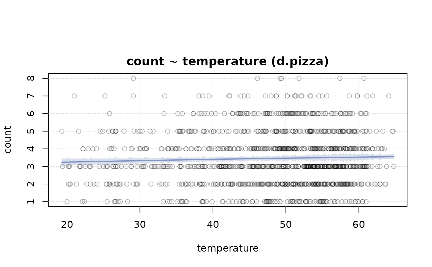 #> ──────────────────────────────────────────────────────────────────────────────
#> count ~ quality (d.pizza)
#>
#> Summary:
#> n pairs: 1'209, valid: 998 (82.5%), missings: 211 (17.5%), groups: 3
#>
#>
#> low medium high
#> mean 3.37013 3.50852 3.39431
#> median 3.00000 3.00000 3.00000
#> sd 1.50360 1.66065 1.50863
#> IQR 2.00000 3.00000 2.00000
#> n 154 352 492
#> np 15.43086% 35.27054% 49.29860%
#> NAs 2 4 4
#> 0s 0 0 0
#>
#> Kruskal-Wallis rank sum test:
#> Kruskal-Wallis chi-squared = 0.7322, df = 2, p-value = 0.6934
#>
#>
#> Warning:
#> Grouping variable contains 201 NAs (16.6%).
#>
#> ──────────────────────────────────────────────────────────────────────────────
#> count ~ quality (d.pizza)
#>
#> Summary:
#> n pairs: 1'209, valid: 998 (82.5%), missings: 211 (17.5%), groups: 3
#>
#>
#> low medium high
#> mean 3.37013 3.50852 3.39431
#> median 3.00000 3.00000 3.00000
#> sd 1.50360 1.66065 1.50863
#> IQR 2.00000 3.00000 2.00000
#> n 154 352 492
#> np 15.43086% 35.27054% 49.29860%
#> NAs 2 4 4
#> 0s 0 0 0
#>
#> Kruskal-Wallis rank sum test:
#> Kruskal-Wallis chi-squared = 0.7322, df = 2, p-value = 0.6934
#>
#>
#> Warning:
#> Grouping variable contains 201 NAs (16.6%).
#>
 #> ──────────────────────────────────────────────────────────────────────────────
#> operator ~ driver (d.pizza)
#>
#> Summary:
#> n: 1'196, rows: 7, columns: 3
#>
#> Pearson's Chi-squared test:
#> X-squared = 133.06, df = 12, p-value < 2.2e-16
#> Log likelihood ratio (G-test) test of independence:
#> G = 133.53, X-squared df = 12, p-value < 2.2e-16
#> Mantel-Haenszel Chi-squared:
#> X-squared = 33.539, df = 1, p-value = 0.000000006984
#>
#> Contingency Coeff. 0.316
#> Cramer's V 0.236
#> Kendall Tau-b -0.145
#>
#>
#> operator Allanah Maria Rhonda Sum
#> driver
#>
#> Butcher freq 30 8 58 96
#> perc 2.5% 0.7% 4.8% 8.0%
#> p.row 31.2% 8.3% 60.4% .
#> p.col 8.3% 2.1% 13.0% .
#>
#> Carpenter freq 58 87 125 270
#> perc 4.8% 7.3% 10.5% 22.6%
#> p.row 21.5% 32.2% 46.3% .
#> p.col 16.0% 22.4% 28.1% .
#>
#> Carter freq 55 117 62 234
#> perc 4.6% 9.8% 5.2% 19.6%
#> p.row 23.5% 50.0% 26.5% .
#> p.col 15.2% 30.2% 13.9% .
#>
#> Farmer freq 28 38 50 116
#> perc 2.3% 3.2% 4.2% 9.7%
#> p.row 24.1% 32.8% 43.1% .
#> p.col 7.7% 9.8% 11.2% .
#>
#> Hunter freq 68 43 45 156
#> perc 5.7% 3.6% 3.8% 13.0%
#> p.row 43.6% 27.6% 28.8% .
#> p.col 18.7% 11.1% 10.1% .
#>
#> Miller freq 25 50 47 122
#> perc 2.1% 4.2% 3.9% 10.2%
#> p.row 20.5% 41.0% 38.5% .
#> p.col 6.9% 12.9% 10.6% .
#>
#> Taylor freq 99 45 58 202
#> perc 8.3% 3.8% 4.8% 16.9%
#> p.row 49.0% 22.3% 28.7% .
#> p.col 27.3% 11.6% 13.0% .
#>
#> Sum freq 363 388 445 1'196
#> perc 30.4% 32.4% 37.2% 100.0%
#> p.row . . . .
#> p.col . . . .
#>
#>
#> ──────────────────────────────────────────────────────────────────────────────
#> operator ~ driver (d.pizza)
#>
#> Summary:
#> n: 1'196, rows: 7, columns: 3
#>
#> Pearson's Chi-squared test:
#> X-squared = 133.06, df = 12, p-value < 2.2e-16
#> Log likelihood ratio (G-test) test of independence:
#> G = 133.53, X-squared df = 12, p-value < 2.2e-16
#> Mantel-Haenszel Chi-squared:
#> X-squared = 33.539, df = 1, p-value = 0.000000006984
#>
#> Contingency Coeff. 0.316
#> Cramer's V 0.236
#> Kendall Tau-b -0.145
#>
#>
#> operator Allanah Maria Rhonda Sum
#> driver
#>
#> Butcher freq 30 8 58 96
#> perc 2.5% 0.7% 4.8% 8.0%
#> p.row 31.2% 8.3% 60.4% .
#> p.col 8.3% 2.1% 13.0% .
#>
#> Carpenter freq 58 87 125 270
#> perc 4.8% 7.3% 10.5% 22.6%
#> p.row 21.5% 32.2% 46.3% .
#> p.col 16.0% 22.4% 28.1% .
#>
#> Carter freq 55 117 62 234
#> perc 4.6% 9.8% 5.2% 19.6%
#> p.row 23.5% 50.0% 26.5% .
#> p.col 15.2% 30.2% 13.9% .
#>
#> Farmer freq 28 38 50 116
#> perc 2.3% 3.2% 4.2% 9.7%
#> p.row 24.1% 32.8% 43.1% .
#> p.col 7.7% 9.8% 11.2% .
#>
#> Hunter freq 68 43 45 156
#> perc 5.7% 3.6% 3.8% 13.0%
#> p.row 43.6% 27.6% 28.8% .
#> p.col 18.7% 11.1% 10.1% .
#>
#> Miller freq 25 50 47 122
#> perc 2.1% 4.2% 3.9% 10.2%
#> p.row 20.5% 41.0% 38.5% .
#> p.col 6.9% 12.9% 10.6% .
#>
#> Taylor freq 99 45 58 202
#> perc 8.3% 3.8% 4.8% 16.9%
#> p.row 49.0% 22.3% 28.7% .
#> p.col 27.3% 11.6% 13.0% .
#>
#> Sum freq 363 388 445 1'196
#> perc 30.4% 32.4% 37.2% 100.0%
#> p.row . . . .
#> p.col . . . .
#>
#>
 #> ──────────────────────────────────────────────────────────────────────────────
#> operator ~ temperature (d.pizza)
#>
#> Summary:
#> n pairs: 1'209, valid: 1'162 (96.1%), missings: 47 (3.9%), groups: 3
#>
#>
#> Allanah Maria Rhonda
#> mean 46.26449 49.26104 48.15127
#> median 48.15000 51.10000 49.70000
#> sd 11.38296 9.64024 8.73639
#> IQR 18.10000 11.95000 10.17500
#> n 352 376 434
#> np 30.29260% 32.35800% 37.34940%
#> NAs 15 12 12
#> 0s 0 0 0
#>
#> Kruskal-Wallis rank sum test:
#> Kruskal-Wallis chi-squared = 11.679, df = 2, p-value = 0.00291
#>
#>
#> Warning:
#> Grouping variable contains 8 NAs (0.662%).
#>
#>
#>
#> Proportions of operator in the quantiles of temperature:
#>
#> Q1 Q2 Q3 Q4
#> Allanah 45.0% 19.9% 22.6% 33.7%
#> Maria 25.8% 31.8% 35.1% 36.8%
#> Rhonda 29.2% 48.3% 42.4% 29.6%
#>
#> ──────────────────────────────────────────────────────────────────────────────
#> operator ~ temperature (d.pizza)
#>
#> Summary:
#> n pairs: 1'209, valid: 1'162 (96.1%), missings: 47 (3.9%), groups: 3
#>
#>
#> Allanah Maria Rhonda
#> mean 46.26449 49.26104 48.15127
#> median 48.15000 51.10000 49.70000
#> sd 11.38296 9.64024 8.73639
#> IQR 18.10000 11.95000 10.17500
#> n 352 376 434
#> np 30.29260% 32.35800% 37.34940%
#> NAs 15 12 12
#> 0s 0 0 0
#>
#> Kruskal-Wallis rank sum test:
#> Kruskal-Wallis chi-squared = 11.679, df = 2, p-value = 0.00291
#>
#>
#> Warning:
#> Grouping variable contains 8 NAs (0.662%).
#>
#>
#>
#> Proportions of operator in the quantiles of temperature:
#>
#> Q1 Q2 Q3 Q4
#> Allanah 45.0% 19.9% 22.6% 33.7%
#> Maria 25.8% 31.8% 35.1% 36.8%
#> Rhonda 29.2% 48.3% 42.4% 29.6%
#>
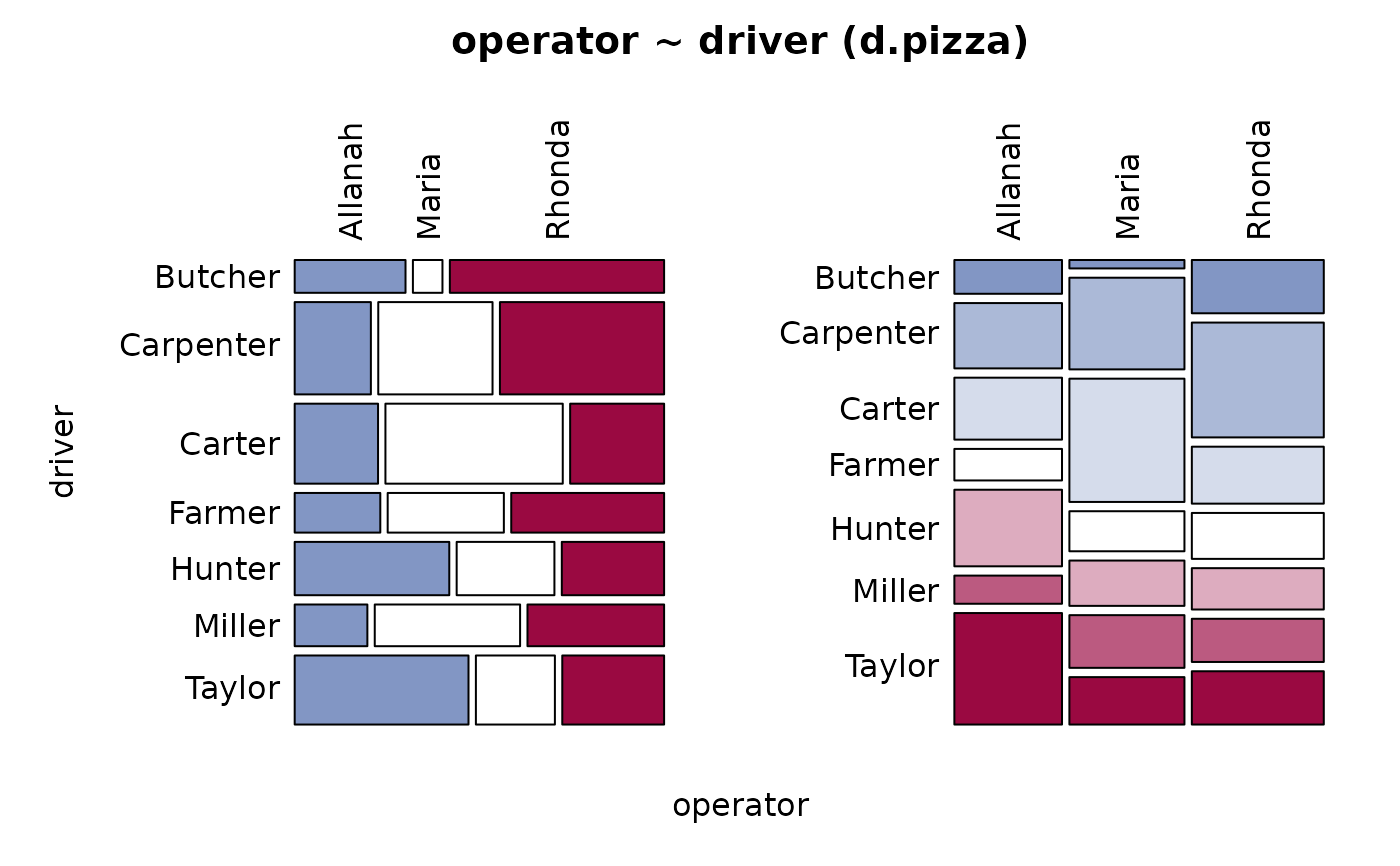 #> Warning: argument 1 does not name a graphical parameter
#> ──────────────────────────────────────────────────────────────────────────────
#> operator ~ wrongpizza (d.pizza)
#>
#> Summary:
#> n: 1'197, rows: 2, columns: 3
#>
#> Pearson's Chi-squared test:
#> X-squared = 113.85, df = 2, p-value < 2.2e-16
#> Log likelihood ratio (G-test) test of independence:
#> G = 108.2, X-squared df = 2, p-value < 2.2e-16
#> Mantel-Haenszel Chi-squared:
#> X-squared = 0.031572, df = 1, p-value = 0.859
#>
#> Contingency Coeff. 0.295
#> Cramer's V 0.308
#> Kendall Tau-b -0.013
#>
#>
#> operator Allanah Maria Rhonda Sum
#> wrongpizza
#>
#> FALSE freq 363 316 436 1'115
#> perc 30.3% 26.4% 36.4% 93.1%
#> p.row 32.6% 28.3% 39.1% .
#> p.col 98.9% 81.9% 98.2% .
#>
#> TRUE freq 4 70 8 82
#> perc 0.3% 5.8% 0.7% 6.9%
#> p.row 4.9% 85.4% 9.8% .
#> p.col 1.1% 18.1% 1.8% .
#>
#> Sum freq 367 386 444 1'197
#> perc 30.7% 32.2% 37.1% 100.0%
#> p.row . . . .
#> p.col . . . .
#>
#>
#> Warning: argument 1 does not name a graphical parameter
#> ──────────────────────────────────────────────────────────────────────────────
#> operator ~ wrongpizza (d.pizza)
#>
#> Summary:
#> n: 1'197, rows: 2, columns: 3
#>
#> Pearson's Chi-squared test:
#> X-squared = 113.85, df = 2, p-value < 2.2e-16
#> Log likelihood ratio (G-test) test of independence:
#> G = 108.2, X-squared df = 2, p-value < 2.2e-16
#> Mantel-Haenszel Chi-squared:
#> X-squared = 0.031572, df = 1, p-value = 0.859
#>
#> Contingency Coeff. 0.295
#> Cramer's V 0.308
#> Kendall Tau-b -0.013
#>
#>
#> operator Allanah Maria Rhonda Sum
#> wrongpizza
#>
#> FALSE freq 363 316 436 1'115
#> perc 30.3% 26.4% 36.4% 93.1%
#> p.row 32.6% 28.3% 39.1% .
#> p.col 98.9% 81.9% 98.2% .
#>
#> TRUE freq 4 70 8 82
#> perc 0.3% 5.8% 0.7% 6.9%
#> p.row 4.9% 85.4% 9.8% .
#> p.col 1.1% 18.1% 1.8% .
#>
#> Sum freq 367 386 444 1'197
#> perc 30.7% 32.2% 37.1% 100.0%
#> p.row . . . .
#> p.col . . . .
#>
#>
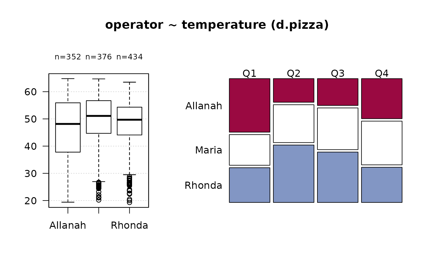 #> ──────────────────────────────────────────────────────────────────────────────
#> operator ~ quality (d.pizza)
#>
#> Summary:
#> n: 1'001, rows: 3, columns: 3
#>
#> Pearson's Chi-squared test:
#> X-squared = 347.23, df = 4, p-value < 2.2e-16
#> Log likelihood ratio (G-test) test of independence:
#> G = 393.18, X-squared df = 4, p-value < 2.2e-16
#> Mantel-Haenszel Chi-squared:
#> X-squared = 61.502, df = 1, p-value = 4.424e-15
#>
#> Contingency Coeff. 0.507
#> Cramer's V 0.416
#> Kendall Tau-b -0.267
#>
#>
#> operator Allanah Maria Rhonda Sum
#> quality
#>
#> low freq 60 3 92 155
#> perc 6.0% 0.3% 9.2% 15.5%
#> p.row 38.7% 1.9% 59.4% .
#> p.col 19.7% 0.9% 24.2% .
#>
#> medium freq 89 39 224 352
#> perc 8.9% 3.9% 22.4% 35.2%
#> p.row 25.3% 11.1% 63.6% .
#> p.col 29.2% 12.3% 58.9% .
#>
#> high freq 156 274 64 494
#> perc 15.6% 27.4% 6.4% 49.4%
#> p.row 31.6% 55.5% 13.0% .
#> p.col 51.1% 86.7% 16.8% .
#>
#> Sum freq 305 316 380 1'001
#> perc 30.5% 31.6% 38.0% 100.0%
#> p.row . . . .
#> p.col . . . .
#>
#>
#> ──────────────────────────────────────────────────────────────────────────────
#> operator ~ quality (d.pizza)
#>
#> Summary:
#> n: 1'001, rows: 3, columns: 3
#>
#> Pearson's Chi-squared test:
#> X-squared = 347.23, df = 4, p-value < 2.2e-16
#> Log likelihood ratio (G-test) test of independence:
#> G = 393.18, X-squared df = 4, p-value < 2.2e-16
#> Mantel-Haenszel Chi-squared:
#> X-squared = 61.502, df = 1, p-value = 4.424e-15
#>
#> Contingency Coeff. 0.507
#> Cramer's V 0.416
#> Kendall Tau-b -0.267
#>
#>
#> operator Allanah Maria Rhonda Sum
#> quality
#>
#> low freq 60 3 92 155
#> perc 6.0% 0.3% 9.2% 15.5%
#> p.row 38.7% 1.9% 59.4% .
#> p.col 19.7% 0.9% 24.2% .
#>
#> medium freq 89 39 224 352
#> perc 8.9% 3.9% 22.4% 35.2%
#> p.row 25.3% 11.1% 63.6% .
#> p.col 29.2% 12.3% 58.9% .
#>
#> high freq 156 274 64 494
#> perc 15.6% 27.4% 6.4% 49.4%
#> p.row 31.6% 55.5% 13.0% .
#> p.col 51.1% 86.7% 16.8% .
#>
#> Sum freq 305 316 380 1'001
#> perc 30.5% 31.6% 38.0% 100.0%
#> p.row . . . .
#> p.col . . . .
#>
#>
 #> ──────────────────────────────────────────────────────────────────────────────
#> driver ~ temperature (d.pizza)
#>
#> Summary:
#> n pairs: 1'209, valid: 1'166 (96.4%), missings: 43 (3.6%), groups: 7
#>
#>
#> Butcher Carpenter Carter Farmer Hunter Miller
#> mean 49.61719 43.49348 50.41925 50.93675 52.14135 47.52397
#> median 51.40000 44.80000 51.75000 54.10000 55.10000 49.60000
#> sd 8.78704 9.40667 8.46700 9.02373 8.88544 8.93474
#> IQR 11.97500 12.50000 11.32500 11.20000 11.57500 8.80000
#> n 96 253 226 117 156 121
#> np 8.23328% 21.69811% 19.38250% 10.03431% 13.37907% 10.37736%
#> NAs 0 19 8 0 0 4
#> 0s 0 0 0 0 0 0
#>
#> Taylor
#> mean 45.09061
#> median 48.50000
#> sd 11.44201
#> IQR 18.40000
#> n 197
#> np 16.89537%
#> NAs 7
#> 0s 0
#>
#> Kruskal-Wallis rank sum test:
#> Kruskal-Wallis chi-squared = 141.93, df = 6, p-value < 2.2e-16
#>
#>
#> Warning:
#> Grouping variable contains 5 NAs (0.414%).
#>
#>
#>
#> Proportions of driver in the quantiles of temperature:
#>
#> Q1 Q2 Q3 Q4
#> Butcher 6.8% 8.1% 7.3% 10.7%
#> Carpenter 34.9% 28.8% 15.9% 6.9%
#> Carter 13.7% 18.3% 21.1% 24.5%
#> Farmer 6.5% 4.7% 14.9% 14.1%
#> Hunter 7.5% 9.5% 11.8% 24.8%
#> Miller 9.2% 12.9% 13.1% 6.2%
#> Taylor 21.2% 17.6% 15.9% 12.8%
#>
#> ──────────────────────────────────────────────────────────────────────────────
#> driver ~ temperature (d.pizza)
#>
#> Summary:
#> n pairs: 1'209, valid: 1'166 (96.4%), missings: 43 (3.6%), groups: 7
#>
#>
#> Butcher Carpenter Carter Farmer Hunter Miller
#> mean 49.61719 43.49348 50.41925 50.93675 52.14135 47.52397
#> median 51.40000 44.80000 51.75000 54.10000 55.10000 49.60000
#> sd 8.78704 9.40667 8.46700 9.02373 8.88544 8.93474
#> IQR 11.97500 12.50000 11.32500 11.20000 11.57500 8.80000
#> n 96 253 226 117 156 121
#> np 8.23328% 21.69811% 19.38250% 10.03431% 13.37907% 10.37736%
#> NAs 0 19 8 0 0 4
#> 0s 0 0 0 0 0 0
#>
#> Taylor
#> mean 45.09061
#> median 48.50000
#> sd 11.44201
#> IQR 18.40000
#> n 197
#> np 16.89537%
#> NAs 7
#> 0s 0
#>
#> Kruskal-Wallis rank sum test:
#> Kruskal-Wallis chi-squared = 141.93, df = 6, p-value < 2.2e-16
#>
#>
#> Warning:
#> Grouping variable contains 5 NAs (0.414%).
#>
#>
#>
#> Proportions of driver in the quantiles of temperature:
#>
#> Q1 Q2 Q3 Q4
#> Butcher 6.8% 8.1% 7.3% 10.7%
#> Carpenter 34.9% 28.8% 15.9% 6.9%
#> Carter 13.7% 18.3% 21.1% 24.5%
#> Farmer 6.5% 4.7% 14.9% 14.1%
#> Hunter 7.5% 9.5% 11.8% 24.8%
#> Miller 9.2% 12.9% 13.1% 6.2%
#> Taylor 21.2% 17.6% 15.9% 12.8%
#>
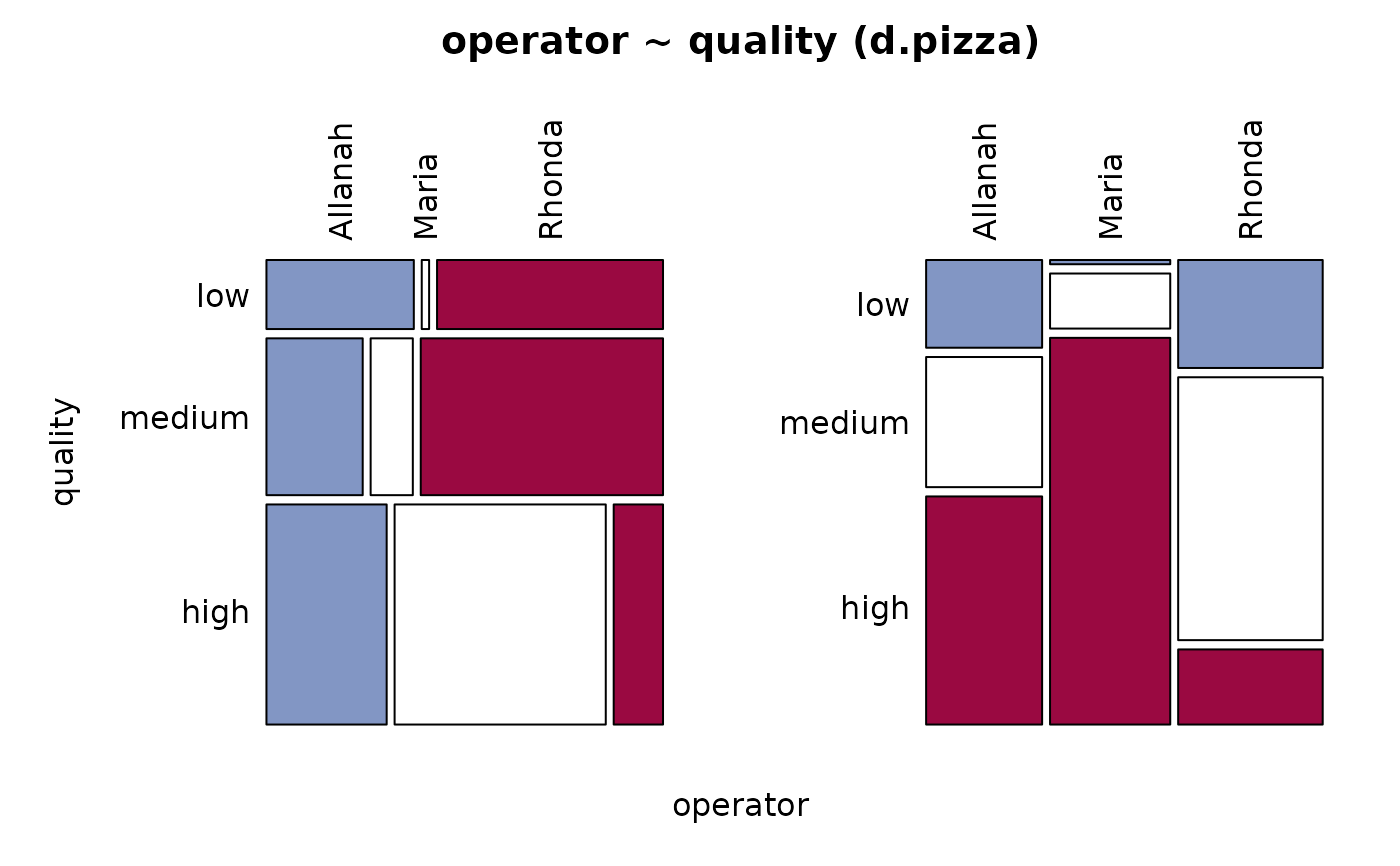 #> Warning: argument 1 does not name a graphical parameter
#> ──────────────────────────────────────────────────────────────────────────────
#> driver ~ wrongpizza (d.pizza)
#>
#> Summary:
#> n: 1'200, rows: 2, columns: 7
#>
#> Pearson's Chi-squared test:
#> X-squared = 14.949, df = 6, p-value = 0.02066
#> Log likelihood ratio (G-test) test of independence:
#> G = 17.11, X-squared df = 6, p-value = 0.008888
#> Mantel-Haenszel Chi-squared:
#> X-squared = 0.16491, df = 1, p-value = 0.6847
#>
#> Contingency Coeff. 0.111
#> Cramer's V 0.112
#> Kendall Tau-b 0.016
#>
#>
#> driver Butcher Carpenter Carter Farmer Hunter Miller
#> wrongpizza
#>
#> FALSE freq 95 252 212 104 149 111
#> perc 7.9% 21.0% 17.7% 8.7% 12.4% 9.2%
#> p.row 8.5% 22.6% 19.0% 9.3% 13.3% 9.9%
#> p.col 99.0% 93.3% 90.6% 90.4% 95.5% 88.8%
#>
#> TRUE freq 1 18 22 11 7 14
#> perc 0.1% 1.5% 1.8% 0.9% 0.6% 1.2%
#> p.row 1.2% 21.7% 26.5% 13.3% 8.4% 16.9%
#> p.col 1.0% 6.7% 9.4% 9.6% 4.5% 11.2%
#>
#> Sum freq 96 270 234 115 156 125
#> perc 8.0% 22.5% 19.5% 9.6% 13.0% 10.4%
#> p.row . . . . . .
#> p.col . . . . . .
#>
#>
#> driver Taylor Sum
#> wrongpizza
#>
#> FALSE freq 194 1'117
#> perc 16.2% 93.1%
#> p.row 17.4% .
#> p.col 95.1% .
#>
#> TRUE freq 10 83
#> perc 0.8% 6.9%
#> p.row 12.0% .
#> p.col 4.9% .
#>
#> Sum freq 204 1'200
#> perc 17.0% 100.0%
#> p.row . .
#> p.col . .
#>
#>
#> Warning: argument 1 does not name a graphical parameter
#> ──────────────────────────────────────────────────────────────────────────────
#> driver ~ wrongpizza (d.pizza)
#>
#> Summary:
#> n: 1'200, rows: 2, columns: 7
#>
#> Pearson's Chi-squared test:
#> X-squared = 14.949, df = 6, p-value = 0.02066
#> Log likelihood ratio (G-test) test of independence:
#> G = 17.11, X-squared df = 6, p-value = 0.008888
#> Mantel-Haenszel Chi-squared:
#> X-squared = 0.16491, df = 1, p-value = 0.6847
#>
#> Contingency Coeff. 0.111
#> Cramer's V 0.112
#> Kendall Tau-b 0.016
#>
#>
#> driver Butcher Carpenter Carter Farmer Hunter Miller
#> wrongpizza
#>
#> FALSE freq 95 252 212 104 149 111
#> perc 7.9% 21.0% 17.7% 8.7% 12.4% 9.2%
#> p.row 8.5% 22.6% 19.0% 9.3% 13.3% 9.9%
#> p.col 99.0% 93.3% 90.6% 90.4% 95.5% 88.8%
#>
#> TRUE freq 1 18 22 11 7 14
#> perc 0.1% 1.5% 1.8% 0.9% 0.6% 1.2%
#> p.row 1.2% 21.7% 26.5% 13.3% 8.4% 16.9%
#> p.col 1.0% 6.7% 9.4% 9.6% 4.5% 11.2%
#>
#> Sum freq 96 270 234 115 156 125
#> perc 8.0% 22.5% 19.5% 9.6% 13.0% 10.4%
#> p.row . . . . . .
#> p.col . . . . . .
#>
#>
#> driver Taylor Sum
#> wrongpizza
#>
#> FALSE freq 194 1'117
#> perc 16.2% 93.1%
#> p.row 17.4% .
#> p.col 95.1% .
#>
#> TRUE freq 10 83
#> perc 0.8% 6.9%
#> p.row 12.0% .
#> p.col 4.9% .
#>
#> Sum freq 204 1'200
#> perc 17.0% 100.0%
#> p.row . .
#> p.col . .
#>
#>
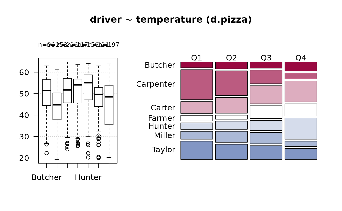 #> ──────────────────────────────────────────────────────────────────────────────
#> driver ~ quality (d.pizza)
#>
#> Summary:
#> n: 1'004, rows: 3, columns: 7
#>
#> Pearson's Chi-squared test:
#> X-squared = 75.29, df = 12, p-value = 0.00000000003238
#> Log likelihood ratio (G-test) test of independence:
#> G = 78.232, X-squared df = 12, p-value = 0.000000000008961
#> Mantel-Haenszel Chi-squared:
#> X-squared = 2.0536, df = 1, p-value = 0.1518
#>
#> Contingency Coeff. 0.264
#> Cramer's V 0.194
#> Kendall Tau-b 0.065
#>
#>
#> driver Butcher Carpenter Carter Farmer Hunter Miller
#> quality
#>
#> low freq 10 59 11 10 8 16
#> perc 1.0% 5.9% 1.1% 1.0% 0.8% 1.6%
#> p.row 6.5% 38.1% 7.1% 6.5% 5.2% 10.3%
#> p.col 12.7% 26.2% 5.6% 10.6% 6.2% 14.7%
#>
#> medium freq 36 90 72 26 43 35
#> perc 3.6% 9.0% 7.2% 2.6% 4.3% 3.5%
#> p.row 10.1% 25.4% 20.3% 7.3% 12.1% 9.9%
#> p.col 45.6% 40.0% 36.7% 27.7% 33.1% 32.1%
#>
#> high freq 33 76 113 58 79 58
#> perc 3.3% 7.6% 11.3% 5.8% 7.9% 5.8%
#> p.row 6.7% 15.4% 22.9% 11.7% 16.0% 11.7%
#> p.col 41.8% 33.8% 57.7% 61.7% 60.8% 53.2%
#>
#> Sum freq 79 225 196 94 130 109
#> perc 7.9% 22.4% 19.5% 9.4% 12.9% 10.9%
#> p.row . . . . . .
#> p.col . . . . . .
#>
#>
#> driver Taylor Sum
#> quality
#>
#> low freq 41 155
#> perc 4.1% 15.4%
#> p.row 26.5% .
#> p.col 24.0% .
#>
#> medium freq 53 355
#> perc 5.3% 35.4%
#> p.row 14.9% .
#> p.col 31.0% .
#>
#> high freq 77 494
#> perc 7.7% 49.2%
#> p.row 15.6% .
#> p.col 45.0% .
#>
#> Sum freq 171 1'004
#> perc 17.0% 100.0%
#> p.row . .
#> p.col . .
#>
#>
#> ──────────────────────────────────────────────────────────────────────────────
#> driver ~ quality (d.pizza)
#>
#> Summary:
#> n: 1'004, rows: 3, columns: 7
#>
#> Pearson's Chi-squared test:
#> X-squared = 75.29, df = 12, p-value = 0.00000000003238
#> Log likelihood ratio (G-test) test of independence:
#> G = 78.232, X-squared df = 12, p-value = 0.000000000008961
#> Mantel-Haenszel Chi-squared:
#> X-squared = 2.0536, df = 1, p-value = 0.1518
#>
#> Contingency Coeff. 0.264
#> Cramer's V 0.194
#> Kendall Tau-b 0.065
#>
#>
#> driver Butcher Carpenter Carter Farmer Hunter Miller
#> quality
#>
#> low freq 10 59 11 10 8 16
#> perc 1.0% 5.9% 1.1% 1.0% 0.8% 1.6%
#> p.row 6.5% 38.1% 7.1% 6.5% 5.2% 10.3%
#> p.col 12.7% 26.2% 5.6% 10.6% 6.2% 14.7%
#>
#> medium freq 36 90 72 26 43 35
#> perc 3.6% 9.0% 7.2% 2.6% 4.3% 3.5%
#> p.row 10.1% 25.4% 20.3% 7.3% 12.1% 9.9%
#> p.col 45.6% 40.0% 36.7% 27.7% 33.1% 32.1%
#>
#> high freq 33 76 113 58 79 58
#> perc 3.3% 7.6% 11.3% 5.8% 7.9% 5.8%
#> p.row 6.7% 15.4% 22.9% 11.7% 16.0% 11.7%
#> p.col 41.8% 33.8% 57.7% 61.7% 60.8% 53.2%
#>
#> Sum freq 79 225 196 94 130 109
#> perc 7.9% 22.4% 19.5% 9.4% 12.9% 10.9%
#> p.row . . . . . .
#> p.col . . . . . .
#>
#>
#> driver Taylor Sum
#> quality
#>
#> low freq 41 155
#> perc 4.1% 15.4%
#> p.row 26.5% .
#> p.col 24.0% .
#>
#> medium freq 53 355
#> perc 5.3% 35.4%
#> p.row 14.9% .
#> p.col 31.0% .
#>
#> high freq 77 494
#> perc 7.7% 49.2%
#> p.row 15.6% .
#> p.col 45.0% .
#>
#> Sum freq 171 1'004
#> perc 17.0% 100.0%
#> p.row . .
#> p.col . .
#>
#>
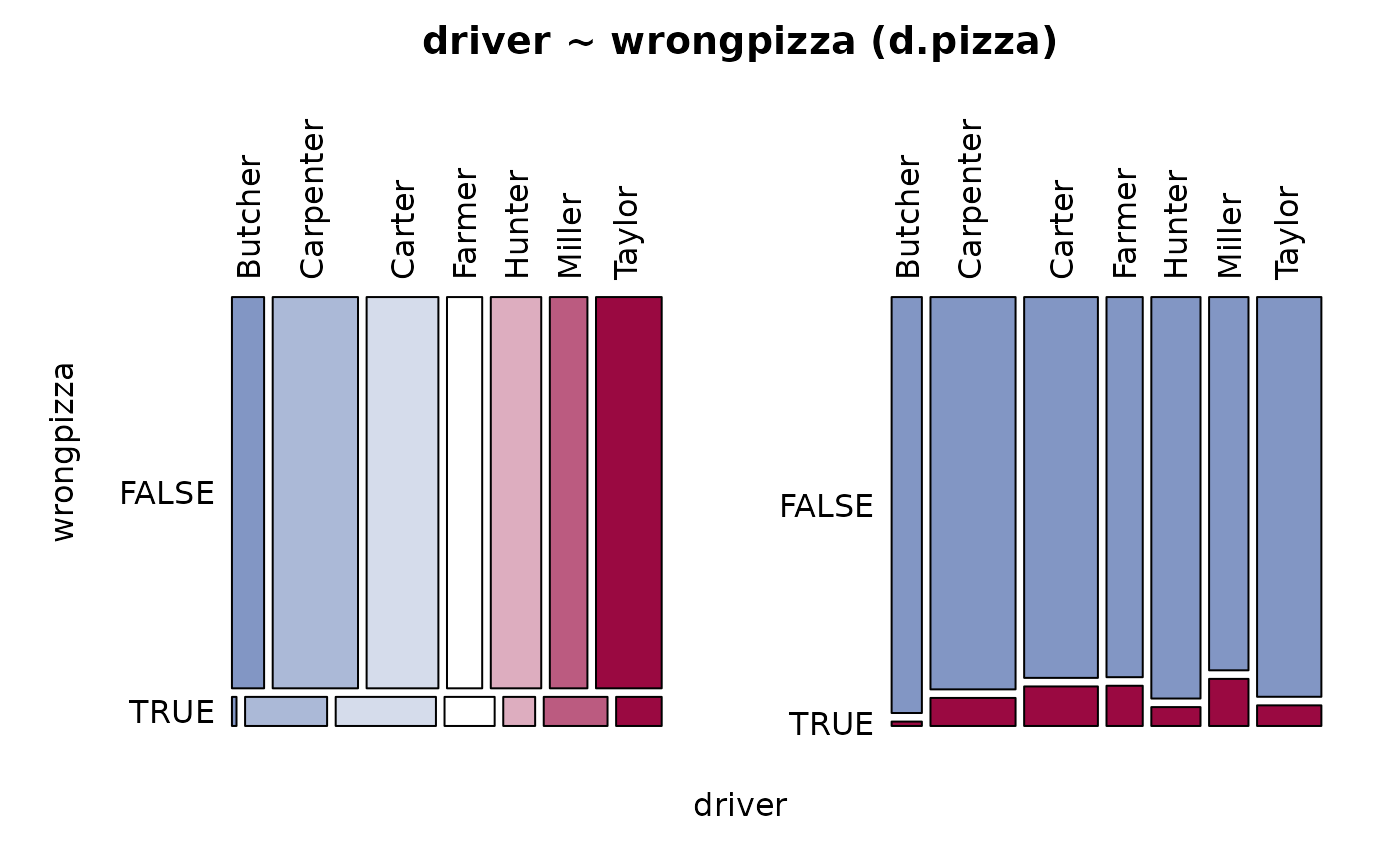 #> ──────────────────────────────────────────────────────────────────────────────
#> temperature ~ wrongpizza (d.pizza)
#>
#> Summary:
#> n pairs: 1'209, valid: 1'166 (96.4%), missings: 43 (3.6%), groups: 2
#>
#>
#> FALSE TRUE
#> mean 47.86667 49.26429
#> median 50.00000 50.40000
#> sd 9.98082 9.04876
#> IQR 13.30000 9.00000
#> n 1'089 77
#> np 93.39623% 6.60377%
#> NAs 33 6
#> 0s 0 0
#>
#> Kruskal-Wallis rank sum test:
#> Kruskal-Wallis chi-squared = 0.86704, df = 1, p-value = 0.3518
#>
#>
#> Warning:
#> Grouping variable contains 4 NAs (0.331%).
#>
#> ──────────────────────────────────────────────────────────────────────────────
#> temperature ~ wrongpizza (d.pizza)
#>
#> Summary:
#> n pairs: 1'209, valid: 1'166 (96.4%), missings: 43 (3.6%), groups: 2
#>
#>
#> FALSE TRUE
#> mean 47.86667 49.26429
#> median 50.00000 50.40000
#> sd 9.98082 9.04876
#> IQR 13.30000 9.00000
#> n 1'089 77
#> np 93.39623% 6.60377%
#> NAs 33 6
#> 0s 0 0
#>
#> Kruskal-Wallis rank sum test:
#> Kruskal-Wallis chi-squared = 0.86704, df = 1, p-value = 0.3518
#>
#>
#> Warning:
#> Grouping variable contains 4 NAs (0.331%).
#>
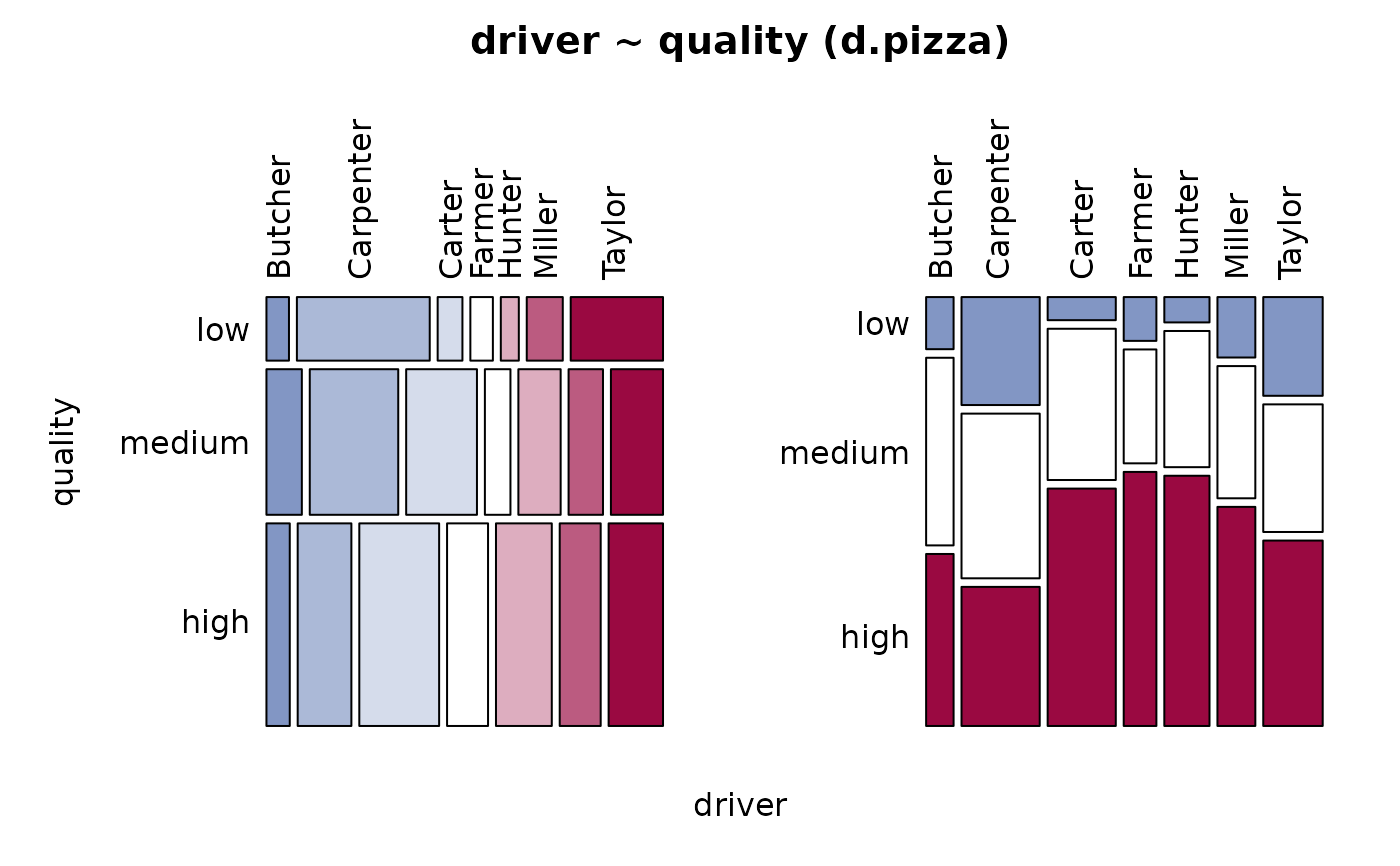 #> ──────────────────────────────────────────────────────────────────────────────
#> temperature ~ quality (d.pizza)
#>
#> Summary:
#> n pairs: 1'209, valid: 974 (80.6%), missings: 235 (19.4%), groups: 3
#>
#>
#> low medium high
#> mean 32.87431 45.64009 53.60436
#> median 32.10000 47.15000 55.15000
#> sd 7.77158 7.38721 6.47392
#> IQR 11.86250 8.50000 8.17500
#> n 144 348 482
#> np 14.78439% 35.72895% 49.48665%
#> NAs 12 8 14
#> 0s 0 0 0
#>
#> Kruskal-Wallis rank sum test:
#> Kruskal-Wallis chi-squared = 461.75, df = 2, p-value < 2.2e-16
#>
#>
#> Warning:
#> Grouping variable contains 201 NAs (16.6%).
#>
#> ──────────────────────────────────────────────────────────────────────────────
#> temperature ~ quality (d.pizza)
#>
#> Summary:
#> n pairs: 1'209, valid: 974 (80.6%), missings: 235 (19.4%), groups: 3
#>
#>
#> low medium high
#> mean 32.87431 45.64009 53.60436
#> median 32.10000 47.15000 55.15000
#> sd 7.77158 7.38721 6.47392
#> IQR 11.86250 8.50000 8.17500
#> n 144 348 482
#> np 14.78439% 35.72895% 49.48665%
#> NAs 12 8 14
#> 0s 0 0 0
#>
#> Kruskal-Wallis rank sum test:
#> Kruskal-Wallis chi-squared = 461.75, df = 2, p-value < 2.2e-16
#>
#>
#> Warning:
#> Grouping variable contains 201 NAs (16.6%).
#>
 #> ──────────────────────────────────────────────────────────────────────────────
#> wrongpizza ~ quality (d.pizza)
#>
#> Summary:
#> n: 1'004, rows: 3, columns: 2
#>
#> Pearson's Chi-squared test:
#> X-squared = 3.5775, df = 2, p-value = 0.1672
#> Log likelihood ratio (G-test) test of independence:
#> G = 3.6034, X-squared df = 2, p-value = 0.165
#> Mantel-Haenszel Chi-squared:
#> X-squared = 0.050237, df = 1, p-value = 0.8227
#>
#> Contingency Coeff. 0.060
#> Cramer's V 0.060
#> Kendall Tau-b 0.001
#>
#>
#> wrongpizza FALSE TRUE Sum
#> quality
#>
#> low freq 141 14 155
#> perc 14.0% 1.4% 15.4%
#> p.row 91.0% 9.0% .
#> p.col 15.0% 21.2% .
#>
#> medium freq 338 17 355
#> perc 33.7% 1.7% 35.4%
#> p.row 95.2% 4.8% .
#> p.col 36.0% 25.8% .
#>
#> high freq 459 35 494
#> perc 45.7% 3.5% 49.2%
#> p.row 92.9% 7.1% .
#> p.col 48.9% 53.0% .
#>
#> Sum freq 938 66 1'004
#> perc 93.4% 6.6% 100.0%
#> p.row . . .
#> p.col . . .
#>
#>
#> ──────────────────────────────────────────────────────────────────────────────
#> wrongpizza ~ quality (d.pizza)
#>
#> Summary:
#> n: 1'004, rows: 3, columns: 2
#>
#> Pearson's Chi-squared test:
#> X-squared = 3.5775, df = 2, p-value = 0.1672
#> Log likelihood ratio (G-test) test of independence:
#> G = 3.6034, X-squared df = 2, p-value = 0.165
#> Mantel-Haenszel Chi-squared:
#> X-squared = 0.050237, df = 1, p-value = 0.8227
#>
#> Contingency Coeff. 0.060
#> Cramer's V 0.060
#> Kendall Tau-b 0.001
#>
#>
#> wrongpizza FALSE TRUE Sum
#> quality
#>
#> low freq 141 14 155
#> perc 14.0% 1.4% 15.4%
#> p.row 91.0% 9.0% .
#> p.col 15.0% 21.2% .
#>
#> medium freq 338 17 355
#> perc 33.7% 1.7% 35.4%
#> p.row 95.2% 4.8% .
#> p.col 36.0% 25.8% .
#>
#> high freq 459 35 494
#> perc 45.7% 3.5% 49.2%
#> p.row 92.9% 7.1% .
#> p.col 48.9% 53.0% .
#>
#> Sum freq 938 66 1'004
#> perc 93.4% 6.6% 100.0%
#> p.row . . .
#> p.col . . .
#>
#>
 # get more flexibility, create the table first
tab <- as.table(apply(HairEyeColor, c(1,2), sum))
tab <- tab[,c("Brown","Hazel","Green","Blue")]
# display only absolute values, row and columnwise percentages
Desc(tab, row.vars=c(3, 1), rfrq="011", plotit=FALSE)
#> ──────────────────────────────────────────────────────────────────────────────
#> tab (table)
#>
#> Summary:
#> n: 592, rows: 4, columns: 4
#>
#> Pearson's Chi-squared test:
#> X-squared = 138.29, df = 9, p-value < 2.2e-16
#> Log likelihood ratio (G-test) test of independence:
#> G = 146.44, X-squared df = 9, p-value < 2.2e-16
#> Mantel-Haenszel Chi-squared:
#> X-squared = 109.64, df = 1, p-value < 2.2e-16
#>
#> Contingency Coeff. 0.435
#> Cramer's V 0.279
#> Kendall Tau-b 0.359
#>
#>
#> Eye Brown Hazel Green Blue Sum
#> Hair
#> freq Black 68 15 5 20 108
#> Brown 119 54 29 84 286
#> Red 26 14 14 17 71
#> Blond 7 10 16 94 127
#> Sum 220 93 64 215 592
#>
#> p.row Black 63.0% 13.9% 4.6% 18.5% .
#> Brown 41.6% 18.9% 10.1% 29.4% .
#> Red 36.6% 19.7% 19.7% 23.9% .
#> Blond 5.5% 7.9% 12.6% 74.0% .
#> Sum 37.2% 15.7% 10.8% 36.3% .
#>
#> p.col Black 30.9% 16.1% 7.8% 9.3% 18.2%
#> Brown 54.1% 58.1% 45.3% 39.1% 48.3%
#> Red 11.8% 15.1% 21.9% 7.9% 12.0%
#> Blond 3.2% 10.8% 25.0% 43.7% 21.5%
#> Sum . . . . .
#>
#>
# do the plot by hand, while setting the colours for the mosaics
cols1 <- SetAlpha(c("sienna4", "burlywood", "chartreuse3", "slategray1"), 0.6)
cols2 <- SetAlpha(c("moccasin", "salmon1", "wheat3", "gray32"), 0.8)
plot(Desc(tab), col1=cols1, col2=cols2)
# get more flexibility, create the table first
tab <- as.table(apply(HairEyeColor, c(1,2), sum))
tab <- tab[,c("Brown","Hazel","Green","Blue")]
# display only absolute values, row and columnwise percentages
Desc(tab, row.vars=c(3, 1), rfrq="011", plotit=FALSE)
#> ──────────────────────────────────────────────────────────────────────────────
#> tab (table)
#>
#> Summary:
#> n: 592, rows: 4, columns: 4
#>
#> Pearson's Chi-squared test:
#> X-squared = 138.29, df = 9, p-value < 2.2e-16
#> Log likelihood ratio (G-test) test of independence:
#> G = 146.44, X-squared df = 9, p-value < 2.2e-16
#> Mantel-Haenszel Chi-squared:
#> X-squared = 109.64, df = 1, p-value < 2.2e-16
#>
#> Contingency Coeff. 0.435
#> Cramer's V 0.279
#> Kendall Tau-b 0.359
#>
#>
#> Eye Brown Hazel Green Blue Sum
#> Hair
#> freq Black 68 15 5 20 108
#> Brown 119 54 29 84 286
#> Red 26 14 14 17 71
#> Blond 7 10 16 94 127
#> Sum 220 93 64 215 592
#>
#> p.row Black 63.0% 13.9% 4.6% 18.5% .
#> Brown 41.6% 18.9% 10.1% 29.4% .
#> Red 36.6% 19.7% 19.7% 23.9% .
#> Blond 5.5% 7.9% 12.6% 74.0% .
#> Sum 37.2% 15.7% 10.8% 36.3% .
#>
#> p.col Black 30.9% 16.1% 7.8% 9.3% 18.2%
#> Brown 54.1% 58.1% 45.3% 39.1% 48.3%
#> Red 11.8% 15.1% 21.9% 7.9% 12.0%
#> Blond 3.2% 10.8% 25.0% 43.7% 21.5%
#> Sum . . . . .
#>
#>
# do the plot by hand, while setting the colours for the mosaics
cols1 <- SetAlpha(c("sienna4", "burlywood", "chartreuse3", "slategray1"), 0.6)
cols2 <- SetAlpha(c("moccasin", "salmon1", "wheat3", "gray32"), 0.8)
plot(Desc(tab), col1=cols1, col2=cols2)
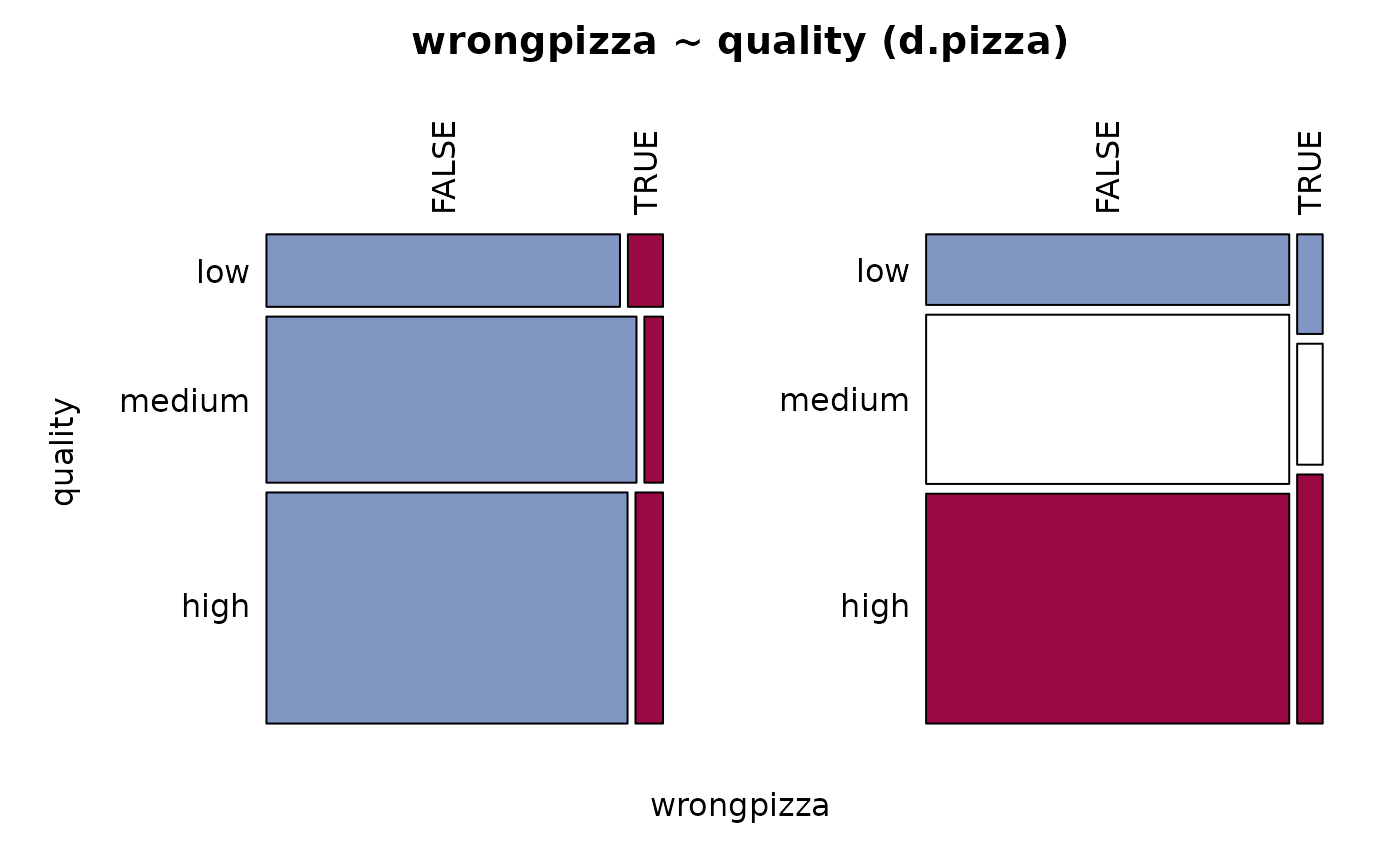 # choose alternative flavours for graphing numeric ~ factor using pipe
# (colors are recyled)
Desc(temperature ~ driver, data = d.pizza) |> plot(type="dens", col=Pal("Tibco"))
# choose alternative flavours for graphing numeric ~ factor using pipe
# (colors are recyled)
Desc(temperature ~ driver, data = d.pizza) |> plot(type="dens", col=Pal("Tibco"))
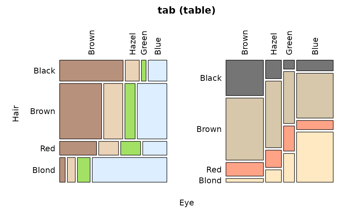 # use global format options for presentation
Fmt(abs=as.fmt(digits=0, big.mark=""))
#> $abs
#> Description: Number format for counts
#> Definition: digits=0, big.mark="'"
#> Example: 314'159
#>
#> $per
#> Description: Percentage number format
#> Definition: digits=1, fmt='%'
#> Example: 31415926.5%
#>
#> $num
#> Description: Number format for floats
#> Definition: digits=3, big.mark="'"
#> Example: 314'159.265
#>
Fmt(per=as.fmt(digits=2, fmt="%"))
#> $abs
#> Description: Number format
#> Definition: digits=0, big.mark=''
#> Example: 314159
#>
#> $per
#> Description: Percentage number format
#> Definition: digits=1, fmt='%'
#> Example: 31415926.5%
#>
#> $num
#> Description: Number format for floating points
#> Definition: digits=0, big.mark="'"
#> Example: 314'159
#>
Desc(area ~ driver, d.pizza, plotit=FALSE)
#> ──────────────────────────────────────────────────────────────────────────────
#> area ~ driver (d.pizza)
#>
#> Summary:
#> n: 1194, rows: 7, columns: 3
#>
#> Pearson's Chi-squared test:
#> X-squared = 1009.5, df = 12, p-value < 2.2e-16
#> Log likelihood ratio (G-test) test of independence:
#> G = 1020.9, X-squared df = 12, p-value < 2.2e-16
#> Mantel-Haenszel Chi-squared:
#> X-squared = 2.6144, df = 1, p-value = 0.1059
#>
#> Contingency Coeff. 0.677
#> Cramer's V 0.650
#> Kendall Tau-b -0.057
#>
#>
#> area Brent Camden Westminster Sum
#> driver
#>
#> Butcher freq 72 1 22 95
#> perc 6.03% 0.08% 1.84% 7.96%
#> p.row 75.79% 1.05% 23.16% .
#> p.col 15.22% 0.29% 5.79% .
#>
#> Carpenter freq 29 19 221 269
#> perc 2.43% 1.59% 18.51% 22.53%
#> p.row 10.78% 7.06% 82.16% .
#> p.col 6.13% 5.57% 58.16% .
#>
#> Carter freq 177 47 5 229
#> perc 14.82% 3.94% 0.42% 19.18%
#> p.row 77.29% 20.52% 2.18% .
#> p.col 37.42% 13.78% 1.32% .
#>
#> Farmer freq 19 87 11 117
#> perc 1.59% 7.29% 0.92% 9.80%
#> p.row 16.24% 74.36% 9.40% .
#> p.col 4.02% 25.51% 2.89% .
#>
#> Hunter freq 128 4 24 156
#> perc 10.72% 0.34% 2.01% 13.07%
#> p.row 82.05% 2.56% 15.38% .
#> p.col 27.06% 1.17% 6.32% .
#>
#> Miller freq 6 41 77 124
#> perc 0.50% 3.43% 6.45% 10.39%
#> p.row 4.84% 33.06% 62.10% .
#> p.col 1.27% 12.02% 20.26% .
#>
#> Taylor freq 42 142 20 204
#> perc 3.52% 11.89% 1.68% 17.09%
#> p.row 20.59% 69.61% 9.80% .
#> p.col 8.88% 41.64% 5.26% .
#>
#> Sum freq 473 341 380 1194
#> perc 39.61% 28.56% 31.83% 100.00%
#> p.row . . . .
#> p.col . . . .
#>
#>
Fmt(abs=as.fmt(digits=0, big.mark="'"))
#> $abs
#> Description: Number format
#> Definition: digits=0, big.mark=''
#> Example: 314159
#>
#> $per
#> Description: Number format
#> Definition: digits=2, fmt='%'
#> Example: 31415926.54%
#>
#> $num
#> Description: Number format for floating points
#> Definition: digits=0, big.mark="'"
#> Example: 314'159
#>
Fmt(per=as.fmt(digits=3, ldigits=0))
#> $abs
#> Description: Number format
#> Definition: digits=0, big.mark="'"
#> Example: 314'159
#>
#> $per
#> Description: Number format
#> Definition: digits=2, fmt='%'
#> Example: 31415926.54%
#>
#> $num
#> Description: Number format for floating points
#> Definition: digits=0, big.mark="'"
#> Example: 314'159
#>
Desc(area ~ driver, d.pizza, plotit=FALSE)
#> ──────────────────────────────────────────────────────────────────────────────
#> area ~ driver (d.pizza)
#>
#> Summary:
#> n: 1'194, rows: 7, columns: 3
#>
#> Pearson's Chi-squared test:
#> X-squared = 1009.5, df = 12, p-value < 2.2e-16
#> Log likelihood ratio (G-test) test of independence:
#> G = 1020.9, X-squared df = 12, p-value < 2.2e-16
#> Mantel-Haenszel Chi-squared:
#> X-squared = 2.6144, df = 1, p-value = 0.1059
#>
#> Contingency Coeff. 0.677
#> Cramer's V 0.650
#> Kendall Tau-b -0.057
#>
#>
#> area Brent Camden Westminster Sum
#> driver
#>
#> Butcher freq 72 1 22 95
#> perc .060 .001 .018 .080
#> p.row .758 .011 .232 .
#> p.col .152 .003 .058 .
#>
#> Carpenter freq 29 19 221 269
#> perc .024 .016 .185 .225
#> p.row .108 .071 .822 .
#> p.col .061 .056 .582 .
#>
#> Carter freq 177 47 5 229
#> perc .148 .039 .004 .192
#> p.row .773 .205 .022 .
#> p.col .374 .138 .013 .
#>
#> Farmer freq 19 87 11 117
#> perc .016 .073 .009 .098
#> p.row .162 .744 .094 .
#> p.col .040 .255 .029 .
#>
#> Hunter freq 128 4 24 156
#> perc .107 .003 .020 .131
#> p.row .821 .026 .154 .
#> p.col .271 .012 .063 .
#>
#> Miller freq 6 41 77 124
#> perc .005 .034 .064 .104
#> p.row .048 .331 .621 .
#> p.col .013 .120 .203 .
#>
#> Taylor freq 42 142 20 204
#> perc .035 .119 .017 .171
#> p.row .206 .696 .098 .
#> p.col .089 .416 .053 .
#>
#> Sum freq 473 341 380 1'194
#> perc .396 .286 .318 1.000
#> p.row . . . .
#> p.col . . . .
#>
#>
# plot arguments can be fixed in detail
z <- Desc(BoxCox(d.pizza$temperature, lambda = 1.5))
plot(z, mar=c(0, 2.1, 4.1, 2.1), args.rug=TRUE, args.hist=list(breaks=50),
args.dens=list(from=0))
# use global format options for presentation
Fmt(abs=as.fmt(digits=0, big.mark=""))
#> $abs
#> Description: Number format for counts
#> Definition: digits=0, big.mark="'"
#> Example: 314'159
#>
#> $per
#> Description: Percentage number format
#> Definition: digits=1, fmt='%'
#> Example: 31415926.5%
#>
#> $num
#> Description: Number format for floats
#> Definition: digits=3, big.mark="'"
#> Example: 314'159.265
#>
Fmt(per=as.fmt(digits=2, fmt="%"))
#> $abs
#> Description: Number format
#> Definition: digits=0, big.mark=''
#> Example: 314159
#>
#> $per
#> Description: Percentage number format
#> Definition: digits=1, fmt='%'
#> Example: 31415926.5%
#>
#> $num
#> Description: Number format for floating points
#> Definition: digits=0, big.mark="'"
#> Example: 314'159
#>
Desc(area ~ driver, d.pizza, plotit=FALSE)
#> ──────────────────────────────────────────────────────────────────────────────
#> area ~ driver (d.pizza)
#>
#> Summary:
#> n: 1194, rows: 7, columns: 3
#>
#> Pearson's Chi-squared test:
#> X-squared = 1009.5, df = 12, p-value < 2.2e-16
#> Log likelihood ratio (G-test) test of independence:
#> G = 1020.9, X-squared df = 12, p-value < 2.2e-16
#> Mantel-Haenszel Chi-squared:
#> X-squared = 2.6144, df = 1, p-value = 0.1059
#>
#> Contingency Coeff. 0.677
#> Cramer's V 0.650
#> Kendall Tau-b -0.057
#>
#>
#> area Brent Camden Westminster Sum
#> driver
#>
#> Butcher freq 72 1 22 95
#> perc 6.03% 0.08% 1.84% 7.96%
#> p.row 75.79% 1.05% 23.16% .
#> p.col 15.22% 0.29% 5.79% .
#>
#> Carpenter freq 29 19 221 269
#> perc 2.43% 1.59% 18.51% 22.53%
#> p.row 10.78% 7.06% 82.16% .
#> p.col 6.13% 5.57% 58.16% .
#>
#> Carter freq 177 47 5 229
#> perc 14.82% 3.94% 0.42% 19.18%
#> p.row 77.29% 20.52% 2.18% .
#> p.col 37.42% 13.78% 1.32% .
#>
#> Farmer freq 19 87 11 117
#> perc 1.59% 7.29% 0.92% 9.80%
#> p.row 16.24% 74.36% 9.40% .
#> p.col 4.02% 25.51% 2.89% .
#>
#> Hunter freq 128 4 24 156
#> perc 10.72% 0.34% 2.01% 13.07%
#> p.row 82.05% 2.56% 15.38% .
#> p.col 27.06% 1.17% 6.32% .
#>
#> Miller freq 6 41 77 124
#> perc 0.50% 3.43% 6.45% 10.39%
#> p.row 4.84% 33.06% 62.10% .
#> p.col 1.27% 12.02% 20.26% .
#>
#> Taylor freq 42 142 20 204
#> perc 3.52% 11.89% 1.68% 17.09%
#> p.row 20.59% 69.61% 9.80% .
#> p.col 8.88% 41.64% 5.26% .
#>
#> Sum freq 473 341 380 1194
#> perc 39.61% 28.56% 31.83% 100.00%
#> p.row . . . .
#> p.col . . . .
#>
#>
Fmt(abs=as.fmt(digits=0, big.mark="'"))
#> $abs
#> Description: Number format
#> Definition: digits=0, big.mark=''
#> Example: 314159
#>
#> $per
#> Description: Number format
#> Definition: digits=2, fmt='%'
#> Example: 31415926.54%
#>
#> $num
#> Description: Number format for floating points
#> Definition: digits=0, big.mark="'"
#> Example: 314'159
#>
Fmt(per=as.fmt(digits=3, ldigits=0))
#> $abs
#> Description: Number format
#> Definition: digits=0, big.mark="'"
#> Example: 314'159
#>
#> $per
#> Description: Number format
#> Definition: digits=2, fmt='%'
#> Example: 31415926.54%
#>
#> $num
#> Description: Number format for floating points
#> Definition: digits=0, big.mark="'"
#> Example: 314'159
#>
Desc(area ~ driver, d.pizza, plotit=FALSE)
#> ──────────────────────────────────────────────────────────────────────────────
#> area ~ driver (d.pizza)
#>
#> Summary:
#> n: 1'194, rows: 7, columns: 3
#>
#> Pearson's Chi-squared test:
#> X-squared = 1009.5, df = 12, p-value < 2.2e-16
#> Log likelihood ratio (G-test) test of independence:
#> G = 1020.9, X-squared df = 12, p-value < 2.2e-16
#> Mantel-Haenszel Chi-squared:
#> X-squared = 2.6144, df = 1, p-value = 0.1059
#>
#> Contingency Coeff. 0.677
#> Cramer's V 0.650
#> Kendall Tau-b -0.057
#>
#>
#> area Brent Camden Westminster Sum
#> driver
#>
#> Butcher freq 72 1 22 95
#> perc .060 .001 .018 .080
#> p.row .758 .011 .232 .
#> p.col .152 .003 .058 .
#>
#> Carpenter freq 29 19 221 269
#> perc .024 .016 .185 .225
#> p.row .108 .071 .822 .
#> p.col .061 .056 .582 .
#>
#> Carter freq 177 47 5 229
#> perc .148 .039 .004 .192
#> p.row .773 .205 .022 .
#> p.col .374 .138 .013 .
#>
#> Farmer freq 19 87 11 117
#> perc .016 .073 .009 .098
#> p.row .162 .744 .094 .
#> p.col .040 .255 .029 .
#>
#> Hunter freq 128 4 24 156
#> perc .107 .003 .020 .131
#> p.row .821 .026 .154 .
#> p.col .271 .012 .063 .
#>
#> Miller freq 6 41 77 124
#> perc .005 .034 .064 .104
#> p.row .048 .331 .621 .
#> p.col .013 .120 .203 .
#>
#> Taylor freq 42 142 20 204
#> perc .035 .119 .017 .171
#> p.row .206 .696 .098 .
#> p.col .089 .416 .053 .
#>
#> Sum freq 473 341 380 1'194
#> perc .396 .286 .318 1.000
#> p.row . . . .
#> p.col . . . .
#>
#>
# plot arguments can be fixed in detail
z <- Desc(BoxCox(d.pizza$temperature, lambda = 1.5))
plot(z, mar=c(0, 2.1, 4.1, 2.1), args.rug=TRUE, args.hist=list(breaks=50),
args.dens=list(from=0))
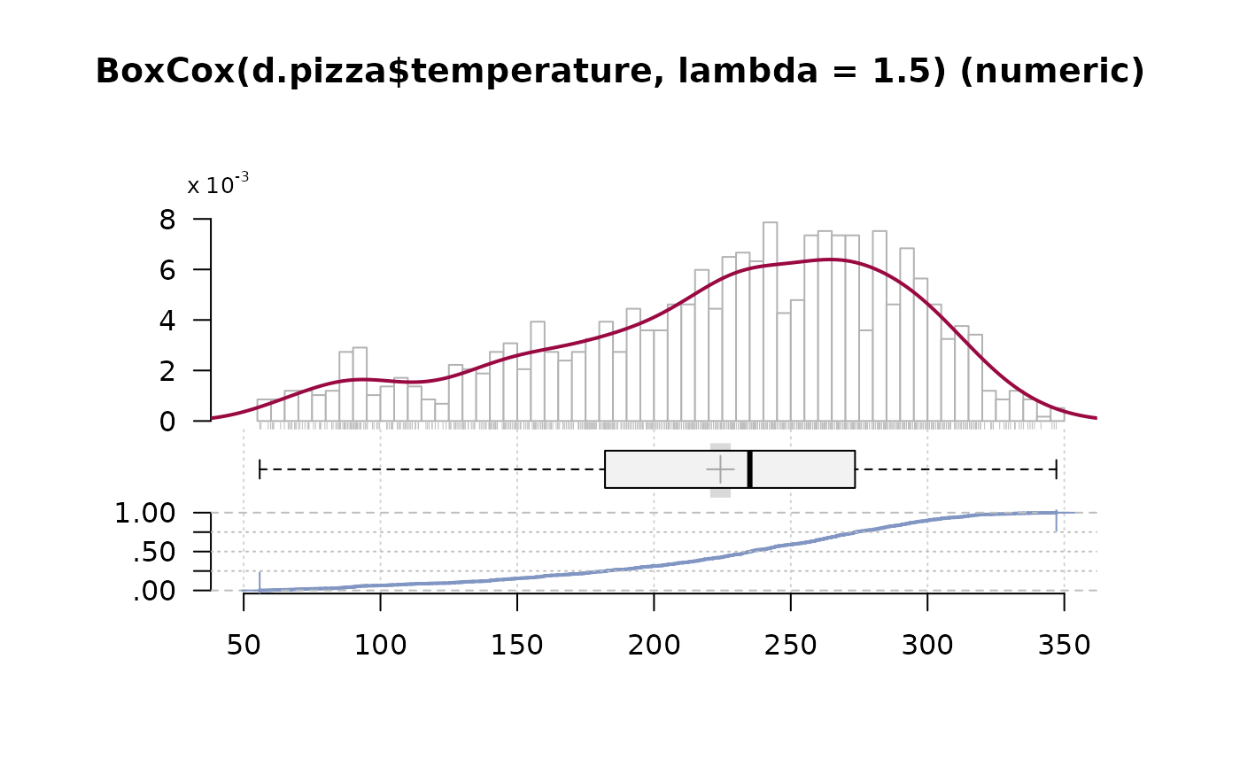 # The default description for count variables can be inappropriate,
# the density curve does not represent the variable well.
set.seed(1972)
x <- rpois(n = 500, lambda = 5)
Desc(x)
#> ──────────────────────────────────────────────────────────────────────────────
#> x (integer)
#>
#> length n NAs unique 0s mean meanCI'
#> 500 500 0 14 4 4.94 4.73
#> 100.0% 0.0% 0.8% 5.14
#>
#> .05 .10 .25 median .75 .90 .95
#> 2.00 2.00 3.00 5.00 6.00 8.00 9.00
#>
#> range sd vcoef mad IQR skew kurt
#> 13.00 2.31 0.47 2.97 3.00 0.45 -0.04
#>
#> lowest : 0 (4), 1 (20), 2 (41), 3 (87), 4 (81)
#> highest: 9 (15), 10 (11), 11 (4), 12 (2), 13
#>
#> heap(?): remarkable frequency (17.4%) for the mode(s) (= 3)
#>
#> ' 95%-CI (classic)
#>
# The default description for count variables can be inappropriate,
# the density curve does not represent the variable well.
set.seed(1972)
x <- rpois(n = 500, lambda = 5)
Desc(x)
#> ──────────────────────────────────────────────────────────────────────────────
#> x (integer)
#>
#> length n NAs unique 0s mean meanCI'
#> 500 500 0 14 4 4.94 4.73
#> 100.0% 0.0% 0.8% 5.14
#>
#> .05 .10 .25 median .75 .90 .95
#> 2.00 2.00 3.00 5.00 6.00 8.00 9.00
#>
#> range sd vcoef mad IQR skew kurt
#> 13.00 2.31 0.47 2.97 3.00 0.45 -0.04
#>
#> lowest : 0 (4), 1 (20), 2 (41), 3 (87), 4 (81)
#> highest: 9 (15), 10 (11), 11 (4), 12 (2), 13
#>
#> heap(?): remarkable frequency (17.4%) for the mode(s) (= 3)
#>
#> ' 95%-CI (classic)
#>
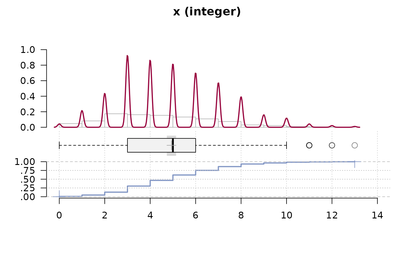 # but setting maxrows to Inf gives a better plot
Desc(x, maxrows = Inf)
#> ──────────────────────────────────────────────────────────────────────────────
#> x (integer)
#>
#> length n NAs unique 0s mean meanCI'
#> 500 500 0 14 4 4.94 4.73
#> 100.0% 0.0% 0.8% 5.14
#>
#> .05 .10 .25 median .75 .90 .95
#> 2.00 2.00 3.00 5.00 6.00 8.00 9.00
#>
#> range sd vcoef mad IQR skew kurt
#> 13.00 2.31 0.47 2.97 3.00 0.45 -0.04
#>
#>
#> value freq perc cumfreq cumperc
#> 1 0 4 .008 4 .008
#> 2 1 20 .040 24 .048
#> 3 2 41 .082 65 .130
#> 4 3 87 .174 152 .304
#> 5 4 81 .162 233 .466
#> 6 5 77 .154 310 .620
#> 7 6 66 .132 376 .752
#> 8 7 54 .108 430 .860
#> 9 8 37 .074 467 .934
#> 10 9 15 .030 482 .964
#> 11 10 11 .022 493 .986
#> 12 11 4 .008 497 .994
#> 13 12 2 .004 499 .998
#> 14 13 1 .002 500 1.000
#>
#> heap(?): remarkable frequency (17.4%) for the mode(s) (= 3)
#>
#> ' 95%-CI (classic)
#>
# but setting maxrows to Inf gives a better plot
Desc(x, maxrows = Inf)
#> ──────────────────────────────────────────────────────────────────────────────
#> x (integer)
#>
#> length n NAs unique 0s mean meanCI'
#> 500 500 0 14 4 4.94 4.73
#> 100.0% 0.0% 0.8% 5.14
#>
#> .05 .10 .25 median .75 .90 .95
#> 2.00 2.00 3.00 5.00 6.00 8.00 9.00
#>
#> range sd vcoef mad IQR skew kurt
#> 13.00 2.31 0.47 2.97 3.00 0.45 -0.04
#>
#>
#> value freq perc cumfreq cumperc
#> 1 0 4 .008 4 .008
#> 2 1 20 .040 24 .048
#> 3 2 41 .082 65 .130
#> 4 3 87 .174 152 .304
#> 5 4 81 .162 233 .466
#> 6 5 77 .154 310 .620
#> 7 6 66 .132 376 .752
#> 8 7 54 .108 430 .860
#> 9 8 37 .074 467 .934
#> 10 9 15 .030 482 .964
#> 11 10 11 .022 493 .986
#> 12 11 4 .008 497 .994
#> 13 12 2 .004 499 .998
#> 14 13 1 .002 500 1.000
#>
#> heap(?): remarkable frequency (17.4%) for the mode(s) (= 3)
#>
#> ' 95%-CI (classic)
#>
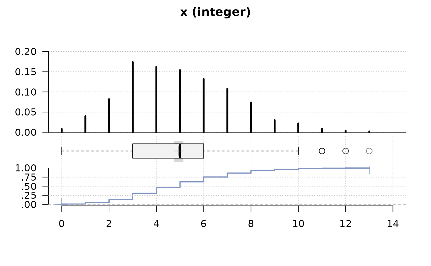 # Output into word document (Windows-specific example) -----------------------
# by simply setting wrd=GetNewWrd()
if (FALSE) { # \dontrun{
# create a new word instance and insert title and contents
wrd <- GetNewWrd(header=TRUE)
# let's have a subset
d.sub <- d.pizza[,c("driver", "date", "operator", "price", "wrongpizza")]
# do just the univariate analysis
Desc(d.sub, wrd=wrd)
} # }
DescToolsOptions(opt)
# Output into word document (Windows-specific example) -----------------------
# by simply setting wrd=GetNewWrd()
if (FALSE) { # \dontrun{
# create a new word instance and insert title and contents
wrd <- GetNewWrd(header=TRUE)
# let's have a subset
d.sub <- d.pizza[,c("driver", "date", "operator", "price", "wrongpizza")]
# do just the univariate analysis
Desc(d.sub, wrd=wrd)
} # }
DescToolsOptions(opt)