Plot Values on a Circular Grid

PlotPolar creates a polar coordinate plot of the radius r in function of the angle theta. 0 degrees is drawn at the 3 o'clock position and angular values increase in a counterclockwise direction.

PlotPolar(r, theta = NULL, type = "p", rlim = NULL, main = "", lwd = par("lwd"),
          lty = par("lty"), col = par("col"), pch = par("pch"), fill = NA,
          cex = par("cex"), mar = c(2, 2, 5, 2), add = FALSE, ...)

Arguments

r: a vector of radial data.
theta: a vector of angular data specified in radians.
type: one out of c("p","l","h"), the plot type, defined following the definition in plot type. "p" means points, "l" will connect the points with lines and "h" is used to plot radial lines from the center to the points.
Default is "p".
rlim: the r limits (r1, r2) of the plot
main: a main title for the plot, see also title.
lwd: a vector of line widths, see par.
lty: a vector of line types, see par.
col: The colors for lines and points. Multiple colors can be specified so that each point can be given its own color. If there are fewer colors than points they are recycled in the standard fashion. Lines will all be plotted in the first colour specified.
pch: a vector of plotting characters or symbols: see points.
fill: fill color, defaults to NA (none).
cex: a numerical vector giving the amount by which plotting characters and symbols should be scaled relative to the default. This works as a multiple of par("cex"). NULL and NA are equivalent to 1.0.
mar: A numerical vector of the form c(bottom, left, top, right) which gives the number of lines of margin to be specified on the four sides of the plot.
add: defines whether points should be added to an existing plot.
...: further arguments are passed to the plot command.

Details

The function is rather flexible and can produce quite a lot of of different plots. So is it also possible to create spider webs or radar plots.

Author

Andri Signorell <andri@signorell.net>

Examples

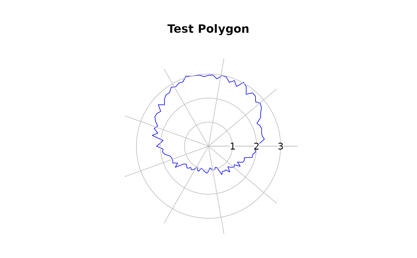
testlen <- c(sin(seq(0, 1.98*pi, length=100))+2+rnorm(100)/10)
testpos <- seq(0, 1.98*pi, length=100)

PlotPolar(testlen, testpos, type="l", main="Test Polygon", col="blue")
PolarGrid(ntheta=9, col="grey", lty="solid", lblradians=TRUE)


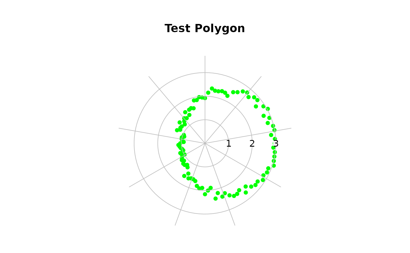
# start at 12 o'clock and plot clockwise
PlotPolar(testlen, -(testpos - pi/2), type="p", main="Test Polygon",
          col="green", pch=16)

PolarGrid(ntheta = rev(seq(0, 2*pi, by=2*pi/9) + pi/2),
          alabels=Format(seq(0, 2*pi, by=2*pi/9), digits=2)[-10], col="grey",
          lty="solid", lblradians=TRUE)



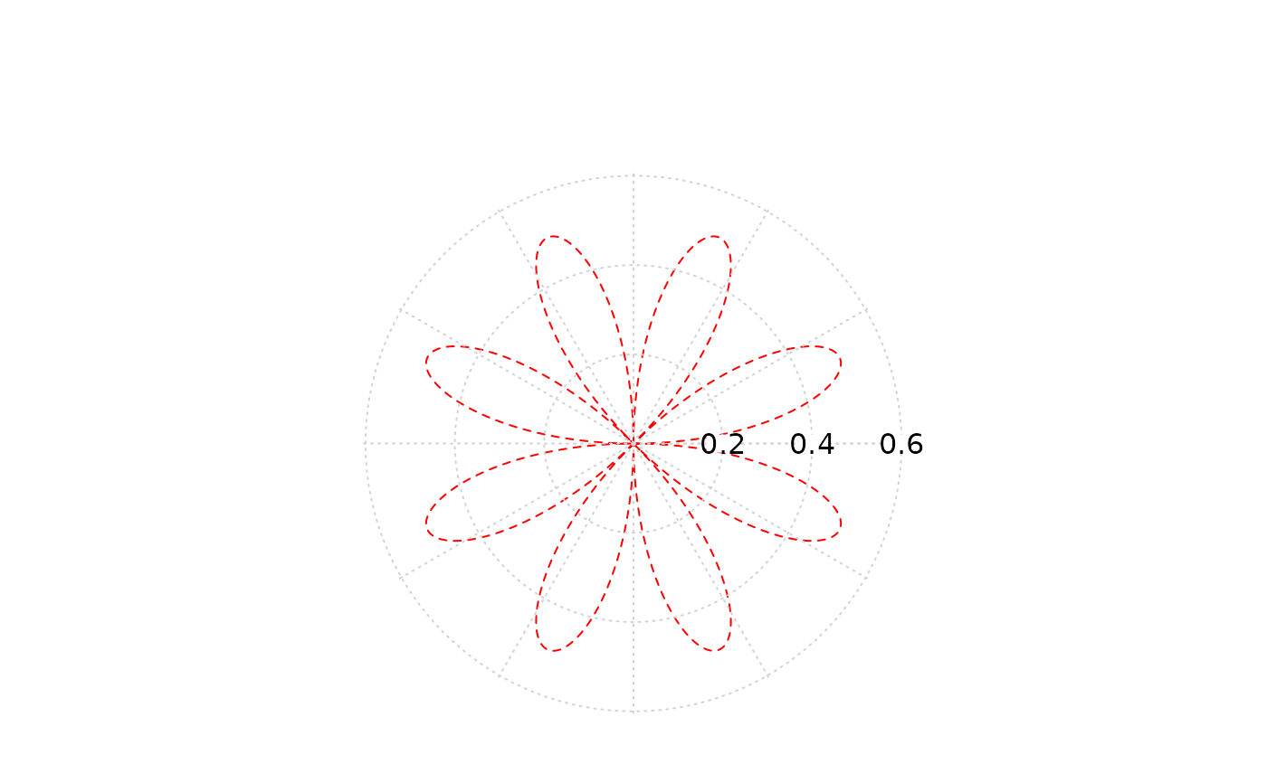
# just because of it's beauty
t <- seq(0,2*pi,0.01)
PlotPolar( r=sin(2*t)*cos(2*t), theta=t, type="l", lty="dashed", col="red" )
PolarGrid()



# use some filled polygons
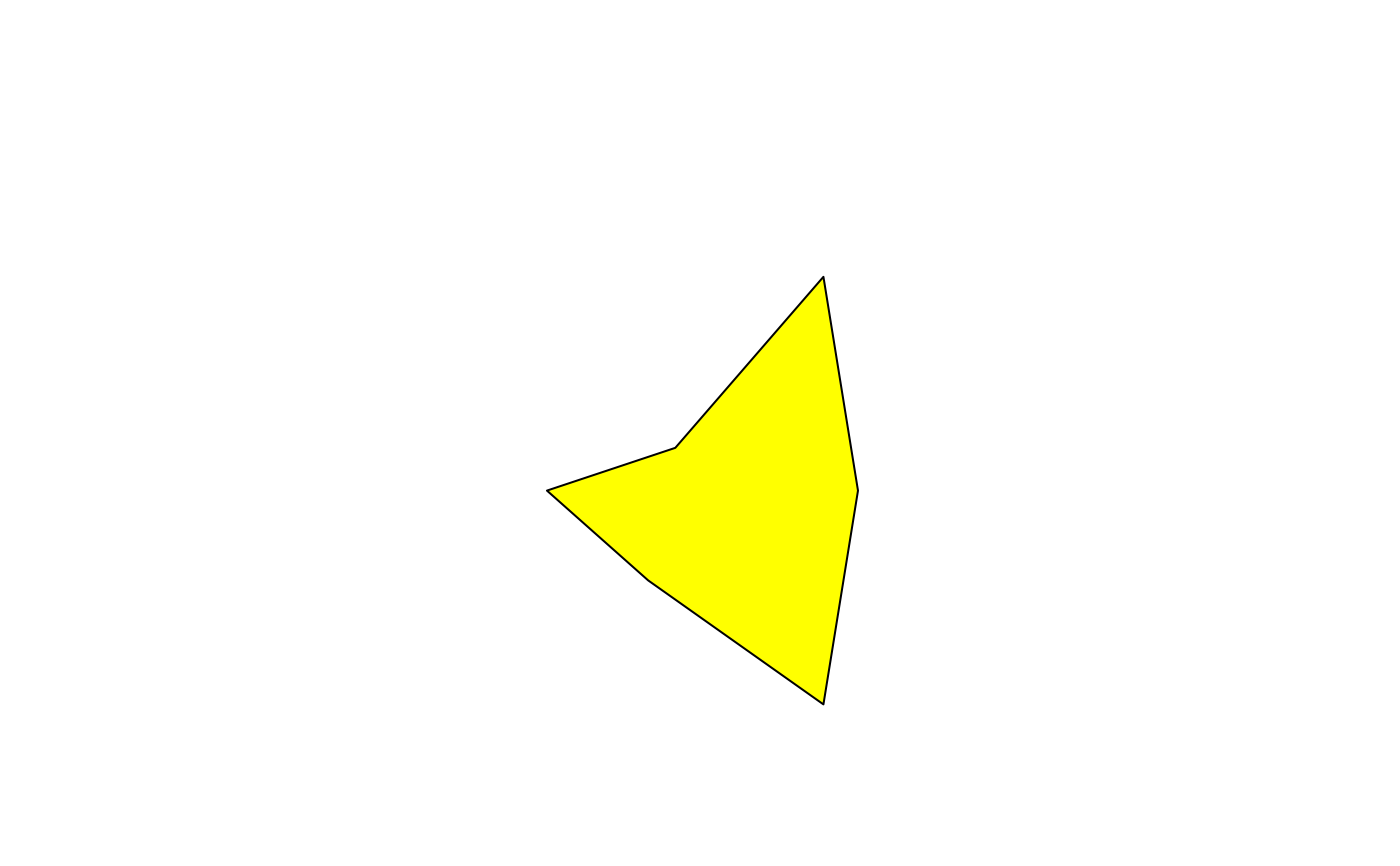
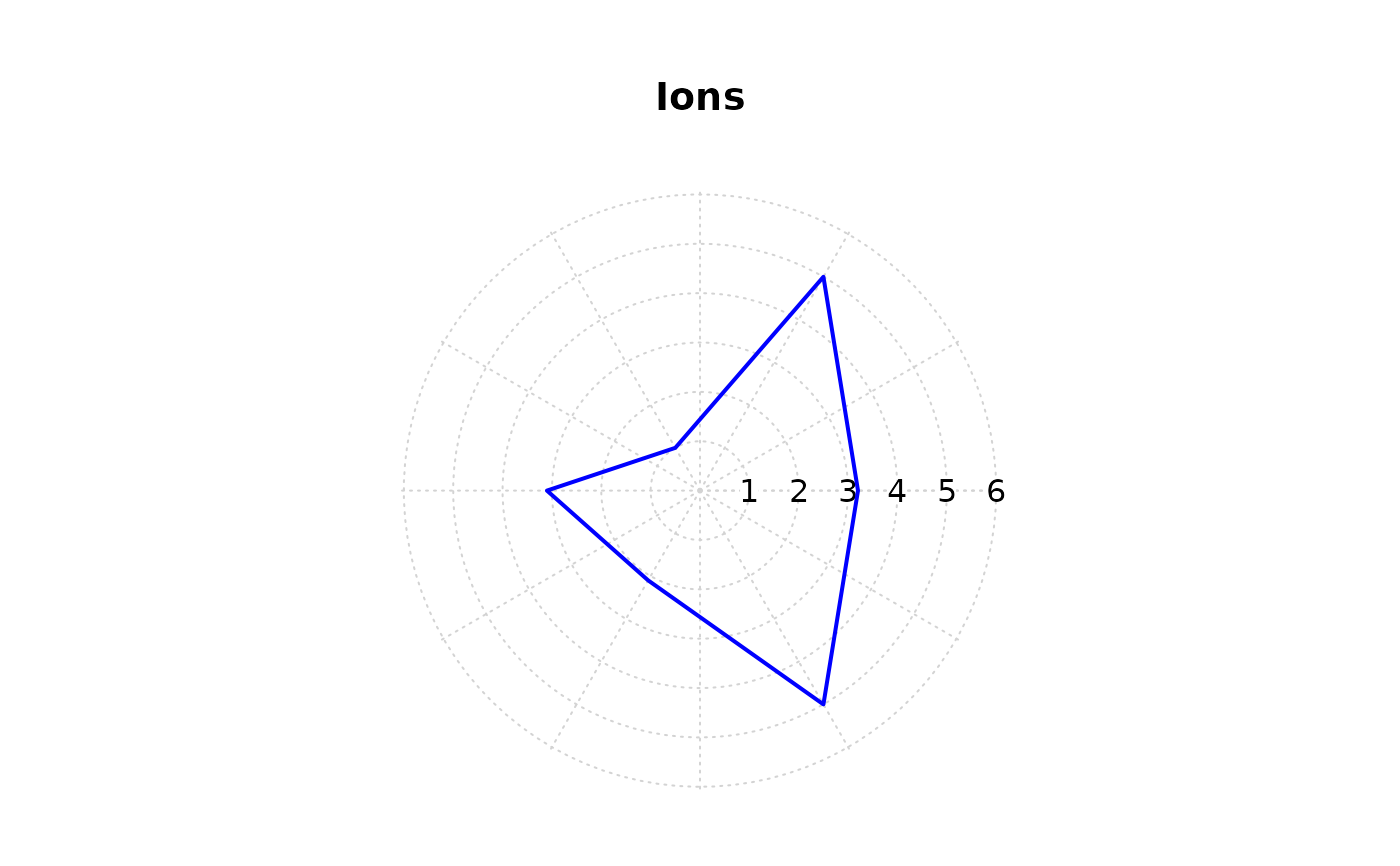
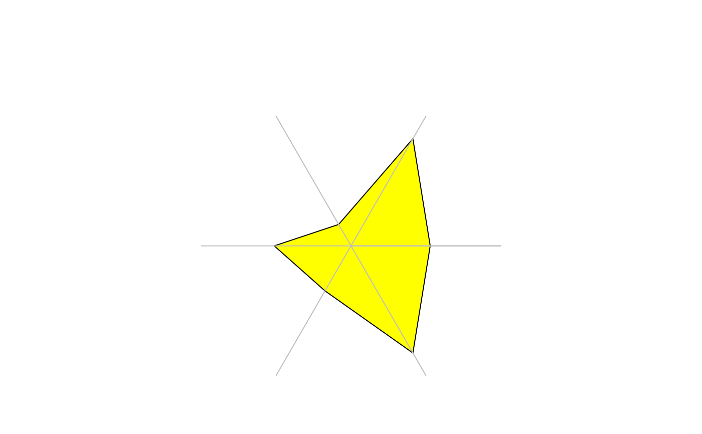
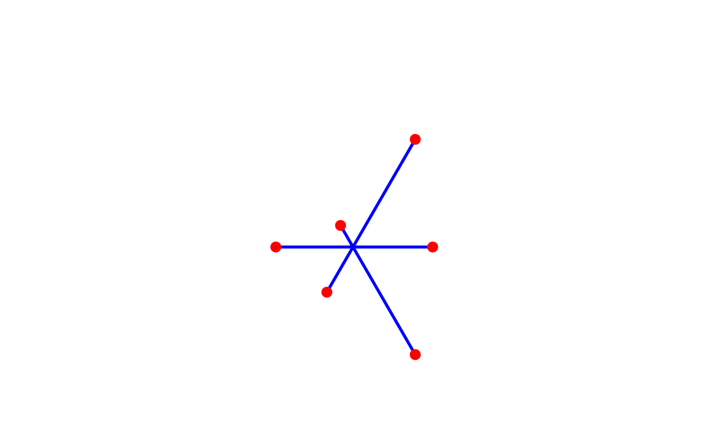
ions <- c(3.2,5,1,3.1,2.1,5)
ion.names <- c("Na","Ca","Mg","Cl","HCO3","SO4")

PlotPolar(r = ions, type="l", fill="yellow")


# the same, but let's have a grid first
PlotPolar(r = ions, type="l", lwd=2, col="blue", main="Ions",
          panel.first=PolarGrid(nr=seq(0, 6, 1)) )


# leave the radial grid out
PlotPolar(r = ions, type="l", fill="yellow")
PolarGrid(nr = NA, ntheta = length(ions), alabels = ion.names,
          col = "grey", lty = "solid" )


# display radial lines
PlotPolar(r = ions, type="h", col="blue", lwd=3)
# add some points
PlotPolar(r = ions, type="p", pch=16, add=TRUE, col="red", cex=1.5)


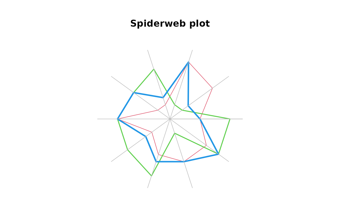
# spiderweb (not really recommended...)
posmat <- matrix(sample(2:9,30,TRUE),nrow=3)
PlotPolar(posmat, type="l", main="Spiderweb plot", col=2:4, lwd=1:3)
PolarGrid(nr=NA, ntheta=ncol(posmat), alabels=paste("X", 1:ncol(posmat), sep=""),
          col="grey", lty="solid" )


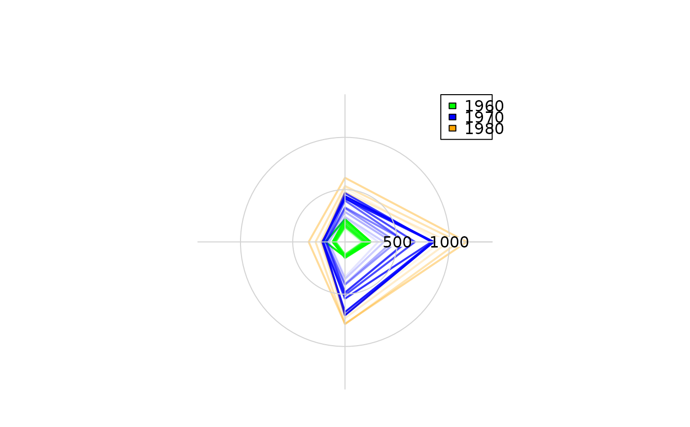
# example from: The grammar of graphics (L. Wilkinson)
data("UKgas")
m <- matrix(UKgas, ncol=4, byrow=TRUE)
cols <- c(SetAlpha(rep("green", 10), seq(0,1,0.1)),
          SetAlpha(rep("blue", 10), seq(0,1,0.1)),
          SetAlpha(rep("orange", 10), seq(0,1,0.1)))
#> Warning: longer argument not a multiple of length of shorter
#> Warning: longer argument not a multiple of length of shorter
#> Warning: longer argument not a multiple of length of shorter

PlotPolar(r=m, type="l", col=cols, lwd=2 )
PolarGrid(ntheta=4, alabels=c("Winter","Spring","Summer","Autumn"), lty="solid")
legend(x="topright", legend=c(1960,1970,1980), fill=c("green","blue","orange"))



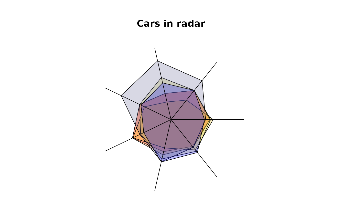
# radarplot (same here, consider alternatives...)
data(mtcars)
d.car <- scale(mtcars[1:6,1:7], center=FALSE)

# let's have a palette with transparent colors (alpha = 32)
cols <- SetAlpha(colorRampPalette(c("red","yellow","blue"), space = "rgb")(6), 0.25)
PlotPolar(d.car, type="l", fill=cols, main="Cars in radar")
PolarGrid(nr=NA, ntheta=ncol(d.car), alabels=colnames(d.car), lty="solid", col="black")


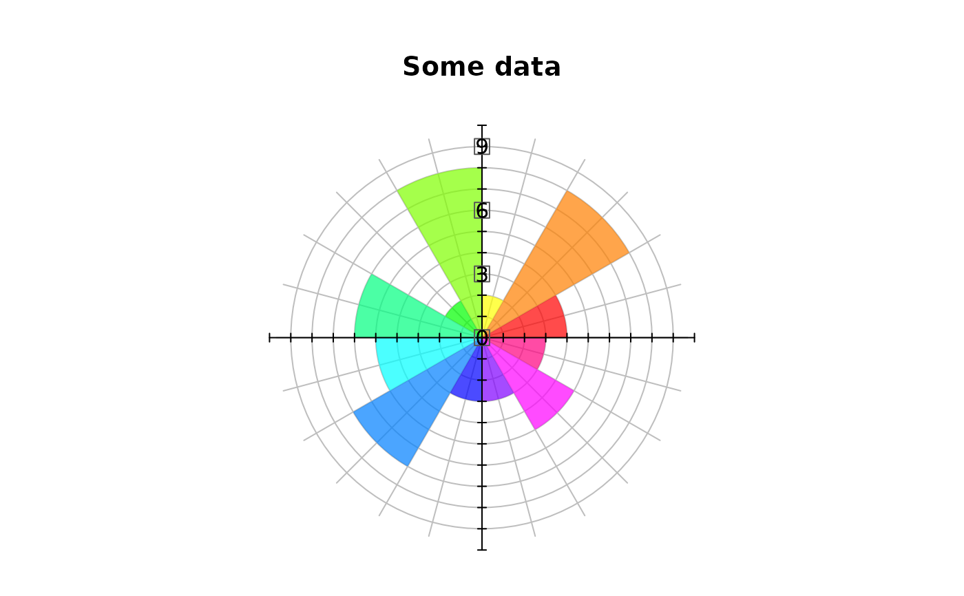
# a polar barplot
x <- c(4,8,2,8,2,6,5,7,3,3,5,3)
theta <- (0:12) * pi / 6
PlotPolar(x, type = "n", main="Some data")
PolarGrid(nr = 0:9, ntheta = 24, col="grey", lty=1, rlabels = NA, alabels = NA)
DrawCircle(x=0, y=0, r.in=0, r.out=x,
                  theta.1 = theta[-length(theta)], theta.2 = theta[-1],
                  col=SetAlpha(rainbow(12), 0.7), border=NA)

segments(x0 = -10:10, y0 = -.2, y1=0.2)
segments(x0=-10, x1=10, y0 = 0)

segments(y0 = -10:10, x0 = -.2, x1=0.2)
segments(y0=-10, y1=10, x0 = 0)

BoxedText(x=0, y=c(0,3,6,9), labels = c(0,3,6,9), xpad = .3, ypad=.3, border="grey35")


# USJudgeRatings
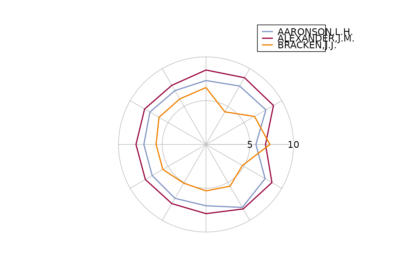
PlotPolar(USJudgeRatings[1,], type="l", col=DescTools::hblue, lwd=2, cex=0.8, 
          panel.first=PolarGrid(ntheta=ncol(USJudgeRatings), col="grey", lty="solid",
                                las=1, alabels=colnames(USJudgeRatings), lblradians=TRUE))
PlotPolar(USJudgeRatings[2,], type="l", col=DescTools::hred, lwd=2, add=TRUE)
PlotPolar(USJudgeRatings[5,], type="l", col=DescTools::horange, lwd=2, add=TRUE)

legend(x="topright", inset=-0.18, 
       col = c(DescTools::hblue, DescTools::hred, DescTools::horange), lwd=2,
       legend=rownames(USJudgeRatings)[c(1, 2, 5)])

Arguments

Details

Author

See also

Examples