Cochran-Armitage Test for Trend
CochranArmitageTest.RdPerform a Cochran Armitage test for trend in binomial proportions across the levels of a single variable. This test is appropriate only when one variable has two levels and the other variable is ordinal. The two-level variable represents the response, and the other represents an explanatory variable with ordered levels. The null hypothesis is the hypothesis of no trend, which means that the binomial proportion is the same for all levels of the explanatory variable.
CochranArmitageTest(x, alternative = c("two.sided", "one.sided"))Arguments
Value
A list of class htest, containing the following components:
- statistic
the z-statistic of the test.
- parameter
the dimension of the table.
- p.value
the p-value for the test.
- alternative
a character string describing the alternative hypothesis.
- method
the character string “Cochran-Armitage test for trend”.
- data.name
a character string giving the names of the data.
References
Agresti, A. (2002) Categorical Data Analysis. John Wiley & Sons
See also
Examples
# http://www.lexjansen.com/pharmasug/2007/sp/sp05.pdf, pp. 4
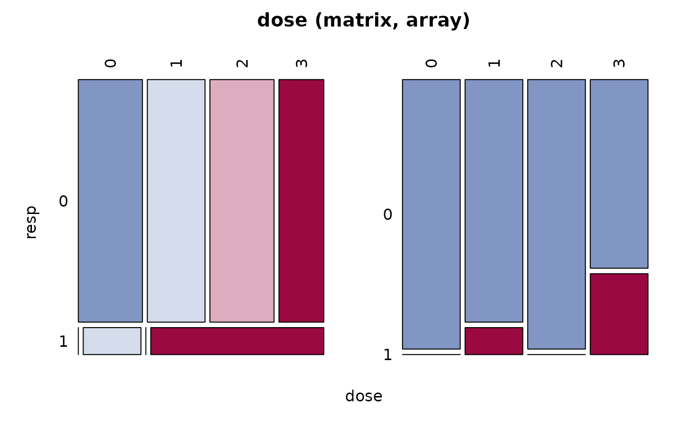
dose <- matrix(c(10,9,10,7, 0,1,0,3), byrow=TRUE, nrow=2, dimnames=list(resp=0:1, dose=0:3))
Desc(dose)
#> ──────────────────────────────────────────────────────────────────────────────
#> dose (matrix, array)
#>
#> Summary:
#> n: 40, rows: 2, columns: 4
#>
#> Pearson's Chi-squared test:
#>   X-squared = 6.6667, df = 3, p-value = 0.08332
#> Log likelihood ratio (G-test) test of independence:
#>   G = 7.2877, X-squared df = 3, p-value = 0.06327
#> Mantel-Haenszel Chi-squared:
#>   X-squared = 3.4667, df = 1, p-value = 0.06262
#>
#> Warning message:
#>   Exp. counts < 5: Chi-squared approx. may be incorrect!!
#>
#>
#> Contingency Coeff.     0.378
#> Cramer's V             0.408
#> Kendall Tau-b          0.272
#>
#>
#>        dose       0      1      2      3    Sum
#> resp
#>
#> 0      freq      10      9     10      7     36
#>        perc   25.0%  22.5%  25.0%  17.5%  90.0%
#>        p.row  27.8%  25.0%  27.8%  19.4%      .
#>        p.col 100.0%  90.0% 100.0%  70.0%      .
#>
#> 1      freq       0      1      0      3      4
#>        perc    0.0%   2.5%   0.0%   7.5%  10.0%
#>        p.row   0.0%  25.0%   0.0%  75.0%      .
#>        p.col   0.0%  10.0%   0.0%  30.0%      .
#>
#> Sum    freq      10     10     10     10     40
#>        perc   25.0%  25.0%  25.0%  25.0% 100.0%
#>        p.row      .      .      .      .      .
#>        p.col      .      .      .      .      .
#>
#>


CochranArmitageTest(dose)
#>
#> 	Cochran-Armitage test for trend
#>
#> data:  dose
#> Z = -1.8856, dim = 4, p-value = 0.05935
#> alternative hypothesis: two.sided
#>
CochranArmitageTest(dose, alternative="one.sided")
#>
#> 	Cochran-Armitage test for trend
#>
#> data:  dose
#> Z = -1.8856, dim = 4, p-value = 0.02967
#> alternative hypothesis: one.sided
#>


# not exactly the same as in package coin:
# independence_test(tumor ~ dose, data = lungtumor, teststat = "quad")
lungtumor <- data.frame(dose = rep(c(0, 1, 2), c(40, 50, 48)),
                        tumor = c(rep(c(0, 1), c(38, 2)),
                                  rep(c(0, 1), c(43, 7)),
                                  rep(c(0, 1), c(33, 15))))
tab <- table(lungtumor$dose, lungtumor$tumor)
CochranArmitageTest(tab)
#>
#> 	Cochran-Armitage test for trend
#>
#> data:  tab
#> Z = -3.2735, dim = 3, p-value = 0.001062
#> alternative hypothesis: two.sided
#>

# but similar to
prop.trend.test(tab[,1], apply(tab,1, sum))
#>
#> 	Chi-squared Test for Trend in Proportions
#>
#> data:  tab[, 1] out of apply(tab, 1, sum) ,
#>  using scores: 1 2 3
#> X-squared = 10.716, df = 1, p-value = 0.001062
#>