Association Measures
Assocs.RdCollects a number of association measures for nominal and ordinal data.
Assocs(x, conf.level = 0.95, verbose = NULL)

# S3 method for class 'Assocs'
print(x, digits = 4, ...)
Arguments
- x
a 2 dimensional contingency table or a matrix.
- conf.level
confidence level of the interval. If set to
NAno confidence interval will be calculated. Default is 0.95.- verbose
integer out of
c(2, 1, 3)defining the verbosity of the reported results. 2 (default) means medium, 1 less and 3 extensive results.
Applies only to tables and is ignored else.- digits
integer which determines the number of digits used in formatting the measures of association.
- ...
further arguments to be passed to or from methods.
Details
This function wraps the association measures phi, contingency coefficient, Cramer's V, Goodman Kruskal's Gamma, Kendall's Tau-b, Stuart's Tau-c, Somers' Delta, Pearson and Spearman correlation, Guttman's Lambda, Theil's Uncertainty Coefficient and the mutual information.
Value
numeric matrix, dimension [1:17, 1:3]
the first column contains the estimate, the second the lower confidence interval, the third the upper one.
See also
Examples
options(scipen=8)
# Example taken from: SAS/STAT(R) 9.2 User's Guide, Second Edition, The FREQ Procedure
# http://support.sas.com/documentation/cdl/en/statugfreq/63124/PDF/default/statugfreq.pdf
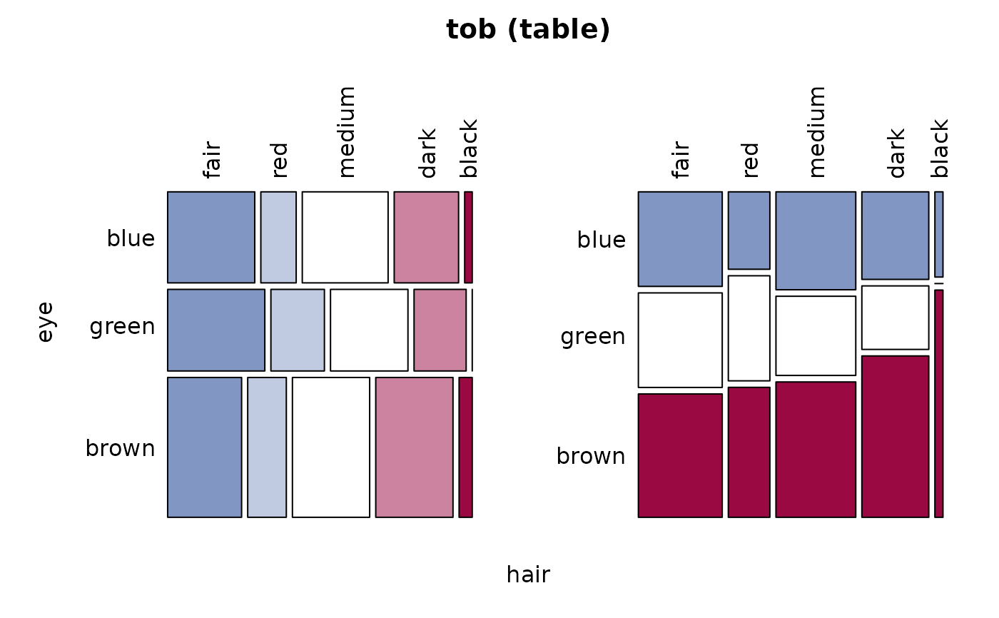
# Hair-Eye-Color pp. 1816
tob <- as.table(matrix(c(
69, 28, 68, 51, 6,
69, 38, 55, 37, 0,
90, 47, 94, 94, 16
), nrow=3, byrow=TRUE,
dimnames=list(eye=c("blue","green","brown"),
hair=c("fair","red","medium","dark","black")) ))
Desc(tob)
#> ──────────────────────────────────────────────────────────────────────────────
#> tob (table)
#>
#> Summary:
#> n: 762, rows: 3, columns: 5
#>
#> Pearson's Chi-squared test:
#> X-squared = 20.925, df = 8, p-value = 0.00735
#> Log likelihood ratio (G-test) test of independence:
#> G = 25.973, X-squared df = 8, p-value = 0.001061
#> Mantel-Haenszel Chi-squared:
#> X-squared = 3.7838, df = 1, p-value = 0.05175
#>
#> Contingency Coeff. 0.163
#> Cramer's V 0.117
#> Kendall Tau-b 0.066
#>
#>
#> hair fair red medium dark black Sum
#> eye
#>
#> blue freq 69 28 68 51 6 222
#> perc 9.1% 3.7% 8.9% 6.7% 0.8% 29.1%
#> p.row 31.1% 12.6% 30.6% 23.0% 2.7% .
#> p.col 30.3% 24.8% 31.3% 28.0% 27.3% .
#>
#> green freq 69 38 55 37 0 199
#> perc 9.1% 5.0% 7.2% 4.9% 0.0% 26.1%
#> p.row 34.7% 19.1% 27.6% 18.6% 0.0% .
#> p.col 30.3% 33.6% 25.3% 20.3% 0.0% .
#>
#> brown freq 90 47 94 94 16 341
#> perc 11.8% 6.2% 12.3% 12.3% 2.1% 44.8%
#> p.row 26.4% 13.8% 27.6% 27.6% 4.7% .
#> p.col 39.5% 41.6% 43.3% 51.6% 72.7% .
#>
#> Sum freq 228 113 217 182 22 762
#> perc 29.9% 14.8% 28.5% 23.9% 2.9% 100.0%
#> p.row . . . . . .
#> p.col . . . . . .
#>
#>
 Assocs(tob)
#> estimate lwr.ci upr.ci
#> Contingency Coeff. 0.1635 - -
#> Cramer V 0.1172 0.0329 0.1500
#> Kendall Tau-b 0.0661 0.0039 0.1284
#> Goodman Kruskal Gamma 0.0949 0.0057 0.1841
#> Stuart Tau-c 0.0691 0.0041 0.1340
#> Somers D C|R 0.0712 0.0042 0.1383
#> Somers D R|C 0.0614 0.0036 0.1192
#> Pearson Correlation 0.0705 -0.0005 0.1408
#> Spearman Correlation 0.0768 0.0058 0.1470
#> Lambda C|R 0.0075 0.0000 0.0571
#> Lambda R|C 0.0000 0.0000 0.0000
#> Lambda sym 0.0042 0.0000 0.0320
#> Uncertainty Coeff. C|R 0.0118 0.0050 0.0186
#> Uncertainty Coeff. R|C 0.0159 0.0067 0.0252
#> Uncertainty Coeff. sym 0.0135 0.0057 0.0214
#> Mutual Information 0.0246 - -
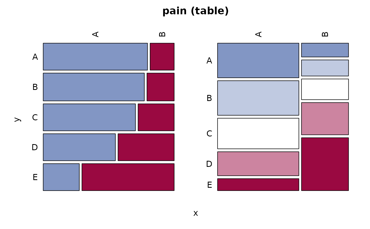
# Example taken from: http://www.math.wpi.edu/saspdf/stat/chap28.pdf
# pp. 1349
pain <- as.table(matrix(c(
26, 6,
26, 7,
23, 9,
18, 14,
9, 23
), ncol=2, byrow=TRUE))
Desc(pain)
#> ──────────────────────────────────────────────────────────────────────────────
#> pain (table)
#>
#> Summary:
#> n: 161, rows: 5, columns: 2
#>
#> Pearson's Chi-squared test:
#> X-squared = 26.603, df = 4, p-value = 0.00002392
#> Log likelihood ratio (G-test) test of independence:
#> G = 26.669, X-squared df = 4, p-value = 0.00002319
#> Mantel-Haenszel Chi-squared:
#> X-squared = 22.819, df = 1, p-value = 0.00000178
#>
#> Contingency Coeff. 0.377
#> Cramer's V 0.406
#> Kendall Tau-b 0.337
#>
#>
#> A B Sum
#>
#> A freq 26 6 32
#> perc 16.1% 3.7% 19.9%
#> p.row 81.2% 18.8% .
#> p.col 25.5% 10.2% .
#>
#> B freq 26 7 33
#> perc 16.1% 4.3% 20.5%
#> p.row 78.8% 21.2% .
#> p.col 25.5% 11.9% .
#>
#> C freq 23 9 32
#> perc 14.3% 5.6% 19.9%
#> p.row 71.9% 28.1% .
#> p.col 22.5% 15.3% .
#>
#> D freq 18 14 32
#> perc 11.2% 8.7% 19.9%
#> p.row 56.2% 43.8% .
#> p.col 17.6% 23.7% .
#>
#> E freq 9 23 32
#> perc 5.6% 14.3% 19.9%
#> p.row 28.1% 71.9% .
#> p.col 8.8% 39.0% .
#>
#> Sum freq 102 59 161
#> perc 63.4% 36.6% 100.0%
#> p.row . . .
#> p.col . . .
#>
#>
Assocs(tob)
#> estimate lwr.ci upr.ci
#> Contingency Coeff. 0.1635 - -
#> Cramer V 0.1172 0.0329 0.1500
#> Kendall Tau-b 0.0661 0.0039 0.1284
#> Goodman Kruskal Gamma 0.0949 0.0057 0.1841
#> Stuart Tau-c 0.0691 0.0041 0.1340
#> Somers D C|R 0.0712 0.0042 0.1383
#> Somers D R|C 0.0614 0.0036 0.1192
#> Pearson Correlation 0.0705 -0.0005 0.1408
#> Spearman Correlation 0.0768 0.0058 0.1470
#> Lambda C|R 0.0075 0.0000 0.0571
#> Lambda R|C 0.0000 0.0000 0.0000
#> Lambda sym 0.0042 0.0000 0.0320
#> Uncertainty Coeff. C|R 0.0118 0.0050 0.0186
#> Uncertainty Coeff. R|C 0.0159 0.0067 0.0252
#> Uncertainty Coeff. sym 0.0135 0.0057 0.0214
#> Mutual Information 0.0246 - -
# Example taken from: http://www.math.wpi.edu/saspdf/stat/chap28.pdf
# pp. 1349
pain <- as.table(matrix(c(
26, 6,
26, 7,
23, 9,
18, 14,
9, 23
), ncol=2, byrow=TRUE))
Desc(pain)
#> ──────────────────────────────────────────────────────────────────────────────
#> pain (table)
#>
#> Summary:
#> n: 161, rows: 5, columns: 2
#>
#> Pearson's Chi-squared test:
#> X-squared = 26.603, df = 4, p-value = 0.00002392
#> Log likelihood ratio (G-test) test of independence:
#> G = 26.669, X-squared df = 4, p-value = 0.00002319
#> Mantel-Haenszel Chi-squared:
#> X-squared = 22.819, df = 1, p-value = 0.00000178
#>
#> Contingency Coeff. 0.377
#> Cramer's V 0.406
#> Kendall Tau-b 0.337
#>
#>
#> A B Sum
#>
#> A freq 26 6 32
#> perc 16.1% 3.7% 19.9%
#> p.row 81.2% 18.8% .
#> p.col 25.5% 10.2% .
#>
#> B freq 26 7 33
#> perc 16.1% 4.3% 20.5%
#> p.row 78.8% 21.2% .
#> p.col 25.5% 11.9% .
#>
#> C freq 23 9 32
#> perc 14.3% 5.6% 19.9%
#> p.row 71.9% 28.1% .
#> p.col 22.5% 15.3% .
#>
#> D freq 18 14 32
#> perc 11.2% 8.7% 19.9%
#> p.row 56.2% 43.8% .
#> p.col 17.6% 23.7% .
#>
#> E freq 9 23 32
#> perc 5.6% 14.3% 19.9%
#> p.row 28.1% 71.9% .
#> p.col 8.8% 39.0% .
#>
#> Sum freq 102 59 161
#> perc 63.4% 36.6% 100.0%
#> p.row . . .
#> p.col . . .
#>
#>
 Assocs(pain)
#> estimate lwr.ci upr.ci
#> Contingency Coeff. 0.3766 - -
#> Cramer V 0.4065 0.2212 0.5411
#> Kendall Tau-b 0.3373 0.2103 0.4642
#> Goodman Kruskal Gamma 0.5313 0.3480 0.7146
#> Stuart Tau-c 0.4111 0.2547 0.5675
#> Somers D C|R 0.2569 0.1592 0.3547
#> Somers D R|C 0.4427 0.2723 0.6130
#> Pearson Correlation 0.3776 0.2368 0.5029
#> Spearman Correlation 0.3771 0.2362 0.5024
#> Lambda C|R 0.2373 0.0732 0.4014
#> Lambda R|C 0.1250 0.0000 0.2547
#> Lambda sym 0.1604 0.0388 0.2821
#> Uncertainty Coeff. C|R 0.1261 0.0346 0.2175
#> Uncertainty Coeff. R|C 0.0515 0.0140 0.0890
#> Uncertainty Coeff. sym 0.0731 0.0199 0.1262
#> Mutual Information 0.1195 - -
Assocs(pain)
#> estimate lwr.ci upr.ci
#> Contingency Coeff. 0.3766 - -
#> Cramer V 0.4065 0.2212 0.5411
#> Kendall Tau-b 0.3373 0.2103 0.4642
#> Goodman Kruskal Gamma 0.5313 0.3480 0.7146
#> Stuart Tau-c 0.4111 0.2547 0.5675
#> Somers D C|R 0.2569 0.1592 0.3547
#> Somers D R|C 0.4427 0.2723 0.6130
#> Pearson Correlation 0.3776 0.2368 0.5029
#> Spearman Correlation 0.3771 0.2362 0.5024
#> Lambda C|R 0.2373 0.0732 0.4014
#> Lambda R|C 0.1250 0.0000 0.2547
#> Lambda sym 0.1604 0.0388 0.2821
#> Uncertainty Coeff. C|R 0.1261 0.0346 0.2175
#> Uncertainty Coeff. R|C 0.0515 0.0140 0.0890
#> Uncertainty Coeff. sym 0.0731 0.0199 0.1262
#> Mutual Information 0.1195 - -