Lorenz Curve

Computes the empirical Lorenz curve for a numeric vector, optionally with weights and grouped via formula interface. Returns an object of class "Lc" (or "LcList" for grouped data) that can be visualized with plot(), lines(), and points() from the pharos package.

Usage

# S3 method for class 'formula'
lc(formula, data, subset, na.action = na.pass, ...)

# Default S3 method
lc(x, n = rep(1, length(x)), na.rm = FALSE, ...)

# S3 method for class 'Lc'
predict(object, newdata, conf.level = NA, general = FALSE, ...)

Arguments

formula: a formula of the form y ~ group specifying the response and grouping variable
data: optional data frame in which to evaluate formula
subset: optional expression indicating which rows of data to use
na.action: function for handling missing values in the model frame. Default is stats::na.pass().
...: further arguments passed to lc.default() from lc.formula(). In predict.Lc(), the argument R (positive integer, default 999) controls the number of bootstrap replications when conf.level is supplied; it is extracted via .extractBootArgs() and ignored otherwise.
x: numeric vector of non-negative values
n: numeric vector of non-negative weights of the same length as x. Defaults to equal weights (rep(1, length(x))).
na.rm: logical. If TRUE, observations with NA in x or n are removed before computation. Default is FALSE.
object: object of class "Lc" as returned by lc()
newdata: optional numeric vector of values in $[0, 1]$ at which to evaluate the Lorenz curve via linear interpolation. If omitted, the original grid points are returned.
conf.level: numeric scalar in $(0, 1)$. If supplied, bootstrap confidence intervals at level conf.level are added as columns lci and uci. Set to NA (default) to suppress intervals.
general: logical. If TRUE, the generalized Lorenz curve is used. Default is FALSE.

Value

lc.default()

an object of class "Lc", a list with components:

p: numeric vector of cumulative population shares starting at 0
L: numeric vector of Lorenz curve values at p
L.general: generalized Lorenz curve values
Gini: estimated Gini coefficient
x: original unsorted data vector
n: original weight vector

lc.formula()

a single "Lc" object if the formula specifies one group, otherwise an object of class "LcList" (a named list of "Lc" objects, one per group level)

predict.Lc()

a data frame with columns p and L (interpolated curve values at newdata). If conf.level is supplied, columns lci and uci are appended.

Details

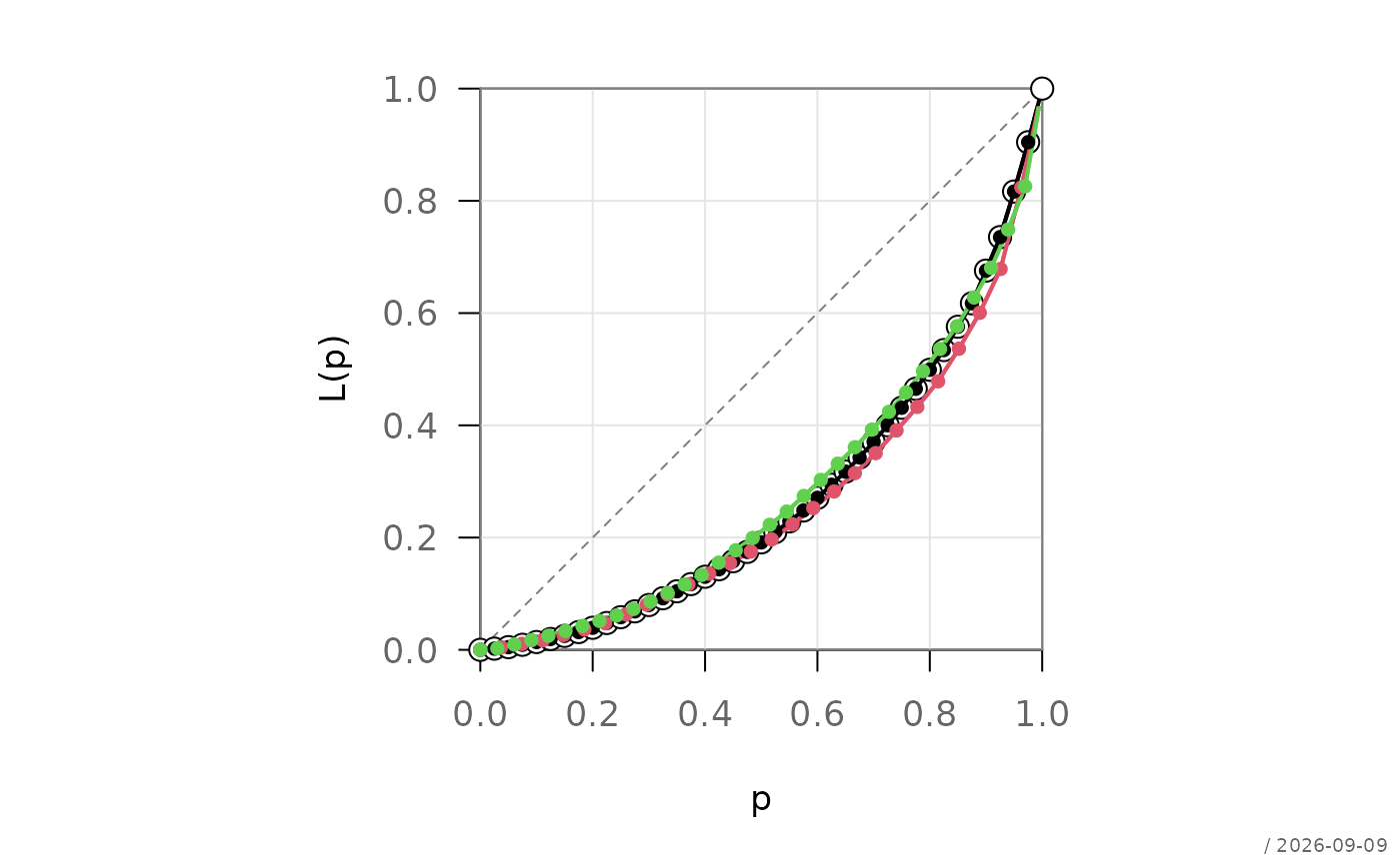
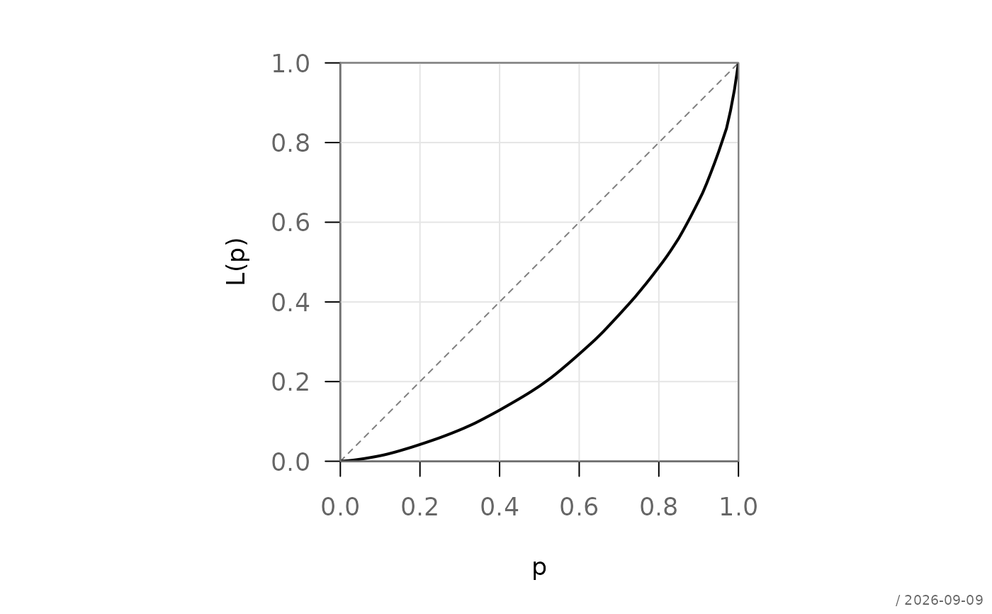
The Lorenz curve is defined as

$$L(p) = \frac{\sum_{i=1}^{k} w_i x_i}{\sum_{i=1}^{n} w_i x_i}$$

where observations are sorted in increasing order and $p$ denotes the cumulative proportion of weights up to rank $k$.

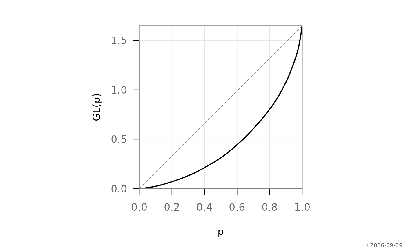
The generalized Lorenz curve scales the standard curve by the weighted mean $\mu$:

$$L_{\text{general}}(p) = L(p) \cdot \mu$$

For formula input of the form y ~ group, the data are split by group and a separate Lorenz curve is computed for each level. A single "Lc" object is returned when there is only one group; otherwise an "LcList".

Bootstrap confidence intervals in predict.Lc() are based on resampling with replacement from the (weighted) empirical distribution, followed by pointwise quantiles across bootstrap replicates. The number of replications is controlled by R passed via ... and extracted by .extractBootArgs() (default R = 999).

References

Lorenz, M. O. (1905). Methods of measuring the concentration of wealth. Publications of the American Statistical Association, 9, 209–219.

Examples

set.seed(1)
x <- rlnorm(100)

# default method
lc_obj <- lc(x)
lc_obj$Gini
#> [1] 0.4697139

# with weights
w <- runif(100, 0.5, 2)
lc(x, n = w)
#> $p
#>   [1] 0.00000000 0.01667602 0.02765357 0.03283079 0.04202449 0.04696748
#>   [7] 0.05638264 0.06201162 0.07023687 0.07523165 0.08742561 0.09825205
#>  [13] 0.10479393 0.11585831 0.12694584 0.14042665 0.14618397 0.15326746
#>  [19] 0.16300758 0.17082749 0.18509908 0.20157914 0.21594853 0.22183435
#>  [25] 0.22653431 0.23381894 0.24359562 0.26002810 0.26771346 0.28102722
#>  [31] 0.29433819 0.30190065 0.31558283 0.32193626 0.33380180 0.34212844
#>  [37] 0.34981967 0.36102089 0.37752414 0.38785057 0.39389959 0.40545989
#>  [43] 0.41644830 0.42900449 0.43735520 0.44582112 0.45861366 0.46531069
#>  [49] 0.47989878 0.49044929 0.49898059 0.51139349 0.51857745 0.52506358
#>  [55] 0.53228217 0.53912207 0.54581827 0.55196081 0.56242497 0.57234343
#>  [61] 0.57840268 0.58761490 0.59325654 0.60751188 0.62296495 0.62811297
#>  [67] 0.63977586 0.64597015 0.65917738 0.66836852 0.67604343 0.68480655
#>  [73] 0.68976904 0.69907536 0.71543905 0.72339506 0.73958177 0.74817614
#>  [79] 0.75419541 0.76442584 0.77049110 0.77698278 0.79373384 0.81034467
#>  [85] 0.81809906 0.83484522 0.84336772 0.85329756 0.86829034 0.88540362
#>  [91] 0.90119921 0.90724790 0.91610539 0.92675580 0.94091655 0.95776753
#>  [97] 0.96870362 0.97654230 0.98229671 0.98884205 1.00000000
#> 
#> $L
#>   [1] 0.000000000 0.001085041 0.001979843 0.002487300 0.003681286 0.004358049
#>   [7] 0.005773725 0.006709560 0.008108789 0.008983490 0.011332336 0.013603296
#>  [13] 0.015135141 0.017994074 0.020902755 0.024723097 0.026409961 0.028490482
#>  [19] 0.031405407 0.033896111 0.038465488 0.043790799 0.048539760 0.050516850
#>  [25] 0.052102875 0.054626241 0.058238004 0.064337495 0.067277383 0.072516484
#>  [31] 0.077864069 0.080985591 0.086993353 0.089786468 0.095274793 0.099484038
#>  [37] 0.103406154 0.109237165 0.117829313 0.123329085 0.126581686 0.133073939
#>  [43] 0.139264704 0.146355201 0.151112877 0.155963733 0.163464595 0.167459882
#>  [49] 0.176400045 0.183172488 0.188650012 0.197272173 0.202416222 0.207084568
#>  [55] 0.212703291 0.218158472 0.223706233 0.228812843 0.237583586 0.246094302
#>  [61] 0.251321895 0.259411254 0.264376006 0.277025077 0.291011623 0.295947191
#>  [67] 0.307262845 0.313703546 0.327461226 0.337143589 0.345277849 0.354735260
#>  [73] 0.360091171 0.370305241 0.388429237 0.397879230 0.417244867 0.427560567
#>  [79] 0.435066080 0.448143516 0.455938312 0.464395391 0.487087777 0.510978938
#>  [85] 0.522562450 0.548207521 0.562912062 0.580689246 0.608207396 0.640751750
#>  [91] 0.671326191 0.683388130 0.703926385 0.730527913 0.767066720 0.812604243
#>  [97] 0.844460949 0.867488643 0.892335058 0.926585892 1.000000000
#> 
#> $L.general
#>   [1] 0.000000000 0.001820792 0.003322346 0.004173902 0.006177514 0.007313179
#>   [7] 0.009688806 0.011259217 0.013607243 0.015075066 0.019016631 0.022827497
#>  [13] 0.025398064 0.030195599 0.035076615 0.041487477 0.044318179 0.047809471
#>  [19] 0.052700966 0.056880580 0.064548386 0.073484714 0.081453878 0.084771605
#>  [25] 0.087433090 0.091667516 0.097728362 0.107963832 0.112897215 0.121688877
#>  [31] 0.130662583 0.135900764 0.145982304 0.150669390 0.159879270 0.166942743
#>  [37] 0.173524392 0.183309327 0.197727688 0.206956777 0.212414920 0.223309477
#>  [43] 0.233698111 0.245596573 0.253580361 0.261720514 0.274307604 0.281012037
#>  [49] 0.296014397 0.307379137 0.316570893 0.331039618 0.339671773 0.347505657
#>  [55] 0.356934357 0.366088618 0.375398236 0.383967565 0.398685623 0.412967336
#>  [61] 0.421739684 0.435314322 0.443645601 0.464871828 0.488342450 0.496624757
#>  [67] 0.515613394 0.526421442 0.549508010 0.565755845 0.579405829 0.595276177
#>  [73] 0.604263853 0.621403939 0.651817558 0.667675456 0.700172655 0.717483284
#>  [79] 0.730078178 0.752023236 0.765103573 0.779295276 0.817375046 0.857466462
#>  [85] 0.876904588 0.919939215 0.944614696 0.974446334 1.020624150 1.075236365
#>  [91] 1.126542898 1.146783866 1.181248818 1.225888462 1.287203712 1.363619581
#>  [97] 1.417077864 1.455720308 1.497414723 1.554890558 1.678085725
#> 
#> $Gini
#> [1] 0.4611728
#> 
#> $x
#>   [1]  0.5344838  1.2015872  0.4336018  4.9297132  1.3902836  0.4402254
#>   [7]  1.6281250  2.0924271  1.7785196  0.7368371  4.5348008  1.4767493
#>  [13]  0.5372775  0.1091863  3.0800041  0.9560610  0.9839401  2.5698209
#>  [19]  2.2732743  1.8110401  2.5067256  2.1861375  1.0774154  0.1367841
#>  [25]  1.8586041  0.9454174  0.8557342  0.2297526  0.6199292  1.5188319
#>  [31]  3.8910520  0.9023185  1.4735458  0.9476168  0.2523194  0.6603439
#>  [37]  0.6741586  0.9424114  3.0042422  2.1450776  0.8482977  0.7761871
#>  [43]  2.0076470  1.7448406  0.5022006  0.4928772  1.4399119  2.1566000
#>  [49]  0.8937348  2.4135718  1.4890017  0.5422509  1.4065216  0.3232391
#>  [55]  4.1913535  7.2456399  0.6926562  0.3519963  1.7677713  0.8736682
#>  [61] 11.0410237  0.9615199  1.9931960  1.0283979  0.4755548  1.2077901
#>  [67]  0.1644813  4.3299451  1.1656202  8.7811877  1.6088337  0.4916705
#>  [73]  1.8417687  0.3929403  0.2854657  1.3383617  0.6419198  1.0011060
#>  [79]  1.0771744  0.5545929  0.5662788  0.8735599  3.2481545  0.2179332
#>  [85]  1.8111214  1.3950781  2.8953322  0.7377252  1.4477618  1.3061695
#>  [91]  0.5812816  3.3463420  3.1912179  2.0141830  4.8882455  1.7480247
#>  [97]  0.2789864  0.5636818  0.2938715  0.6228805
#> 
#> $n
#>   [1] 0.9012623 0.8279679 1.2751953 0.9034259 0.7717525 1.2778642 1.3441744
#>   [8] 0.6937353 0.8845514 1.5769029 1.9421149 0.6502113 1.6448340 1.9219495
#>  [15] 1.7279520 0.9624385 1.4743692 1.9300332 1.9305990 1.0099688 0.8937112
#>  [22] 0.7481809 0.9832521 1.2651878 1.8859527 1.2664395 0.8864319 0.5696913
#>  [29] 1.1267844 1.7810023 1.0208460 0.6971635 1.0617303 1.4471303 1.0851184
#>  [36] 1.5344418 1.5341201 1.3323509 1.1444366 1.1790801 0.9596649 1.3675309
#>  [43] 1.8655555 0.7139061 1.1225714 0.8163886 1.1431256 0.6990350 1.1901447
#>  [50] 1.9144356 1.6429608 1.8993647 1.2060177 1.4053821 1.2274845 0.6632095
#>  [57] 0.8715902 1.2477718 1.0593001 1.9020371 1.2859791 0.9757170 0.9169490
#>  [64] 1.6813108 1.5536938 0.7475415 0.5966863 1.6320584 1.4306150 0.7543652
#>  [71] 0.5933211 0.6635439 1.0725745 0.7539664 0.9479788 0.7883143 0.8857550
#>  [78] 0.7718477 1.2159706 1.6561056 0.5416807 1.2909662 1.8204786 1.0595951
#>  [85] 0.5719387 0.7079424 0.9822382 0.7322474 0.6983423 0.8319589 0.8395712
#>  [92] 0.6971248 1.9723452 0.9905206 1.2604092 1.5221638 0.6487537 0.6783538
#>  [99] 0.5756595 1.8938809
#> 
#> attr(,"class")
#> [1] "Lc"

# formula interface: grouped Lorenz curves
g <- sample(letters[1:3], 100, replace = TRUE)
d <- data.frame(x = x, g = g)
lc_grp <- lc(x ~ g, data = d)

# prediction on a regular grid
predict(lc_obj, newdata = seq(0, 1, by = 0.1))
#>      p          L
#> 1  0.0 0.00000000
#> 2  0.1 0.01389973
#> 3  0.2 0.04211635
#> 4  0.3 0.07866843
#> 5  0.4 0.12834024
#> 6  0.5 0.18850553
#> 7  0.6 0.26915653
#> 8  0.7 0.36760751
#> 9  0.8 0.48726826
#> 10 0.9 0.65324173
#> 11 1.0 1.00000000

# with 95% bootstrap confidence intervals (R = 200 for speed)
predict(lc_obj, newdata = seq(0, 1, by = 0.25),
        conf.level = 0.95, R = 200)
#>      p          L        lci        uci
#> 1 0.00 0.00000000 0.00000000 0.00000000
#> 2 0.25 0.05914571 0.05797344 0.05797344
#> 3 0.50 0.18850553 0.19951495 0.19951495
#> 4 0.75 0.42410184 0.44869940 0.44869940
#> 5 1.00 1.00000000 1.00000000 1.00000000
        
        
# plotting routines from package pharos         
set.seed(1)
x <- rlnorm(100)
lc_obj <- lc(x)

# basic plot
plot(lc_obj)

# overlay confidence band
lines(lc_obj, cbandArgs = list(conf.level = 0.95))

# add points
points(lc_obj, pch = 16)


# generalized Lorenz curve
plot(lc_obj, general = TRUE)


# grouped Lorenz curves
g <- sample(letters[1:3], 100, replace = TRUE)
lc_grp <- lc(x ~ g)
plot(lc_grp)
lines(lc_grp)
points(lc_grp, pch = 16)