Reverse Gumbel Distribution

Density, distribution function, quantile function and random generation for the “Reverse” Gumbel distribution with parameters loc and scale.

Usage

drevgumbel(x, loc = 0, scale = 1, log = FALSE)

prevgumbel(q, loc = 0, scale = 1, lower.tail = TRUE, log.p = FALSE)

qrevgumbel(p, loc = 0, scale = 1, lower.tail = TRUE, log.p = FALSE)

rrevgumbel(n, loc = 0, scale = 1)

qrevgumbelExp(p, loc = 0, scale = 1, lower.tail = TRUE, log.p = FALSE)

Arguments

x, q: numeric vector of abscissa (or quantile) values at which to evaluate the density or distribution function.
loc: location of the distribution.
scale: scale ($> 0$) of the distribution.
log, log.p: logical; if TRUE, probabilities p are given as log(p) and the density is returned on the log scale.
lower.tail: logical; if TRUE (default), probabilities are P[X <= x], otherwise, P[X > x].
p: numeric vector of probabilities at which to evaluate the quantile function.
n: number of random variates, i.e., length() of resulting vector of rrevgumbel().

Value

A numeric vector, of the same length as x, q, or p for the first three functions, and of length n for rrevgumbel(). qrevgumbelExp() gives the quantiles of $\exp(X)$, the exponential parametrization used in some applications.

Details

The reverse Gumbel distribution is the distribution of $a - bY$ for a standard Gumbel $Y$, i.e. the Type I extreme value distribution for minima. With $`loc` = a$ and $`scale` = b$ its distribution function is $$F(x) = 1 - \exp\left\{-\exp\left[\left(\frac{x-a}{b}\right)\right]\right\}$$ for all real $x$, where $b > 0$.

Note

Based on code by Werner Stahel, partly inspired by the VGAM package (numeric refinements by Martin Maechler), adapted to conform to package standards.

Examples


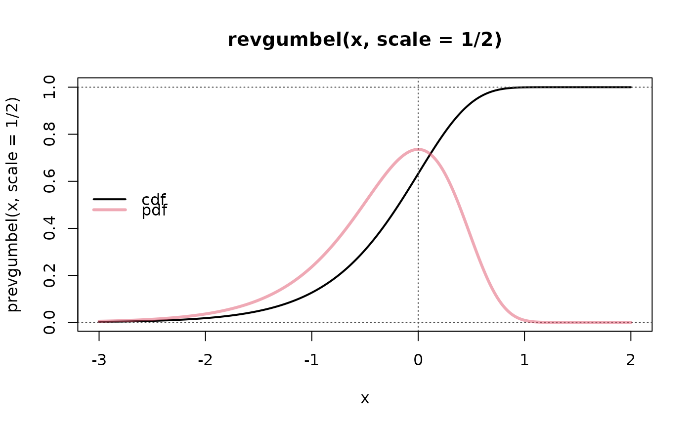
curve(prevgumbel(x, scale= 1/2), -3,2, n=1001, col=1, lwd=2,
      main = "revgumbel(x, scale = 1/2)")
abline(h=0:1, v = 0, lty=3, col = "gray30")
curve(drevgumbel(x, scale= 1/2),       n=1001, add=TRUE,
      col = (col.d <- adjustcolor(2, 0.5)), lwd=3)
legend("left", c("cdf","pdf"), col=c("black", col.d), lwd=2:3, bty="n")


med <- qrevgumbel(0.5, scale=1/2)
cat("The median is:",  format(med),"\n")
#> The median is: -0.1832565