This function was developed to create a univariate graphical representation
of the frequency distribution of a numerical vector.
It combines a histogram, a density
curve, a boxplot and the empirical cumulative distribution function (ecdf)
in one single plot. A rug as well as a model distribution curve (e.g. a
normal curve) can optionally be superposed. This results in a dense and
informative picture of the facts. Still the function remains flexible as all
possible arguments can be passed to the single components (hist,
boxplot etc.) as a list (see examples).
PlotFdist(
  x,
  main = deparse(substitute(x)),
  xlab = "",
  xlim = NULL,
  args.hist = NULL,
  args.rug = NA,
  args.dens = NULL,
  args.curve = NA,
  args.boxplot = NULL,
  args.ecdf = NULL,
  args.curve.ecdf = NA,
  heights = NULL,
  pdist = NULL,
  na.rm = FALSE,
  cex.axis = NULL,
  cex.main = NULL,
  mar = NULL,
  las = 1
)
Arguments
- x
the numerical variable, whose distribution is to be plotted.
- main
main title of the plot.
- xlab
label of the x-axis, defaults to
"". (The name of the variable is typically placed in the main title and would be redundant here.)- xlim
range of the x-axis, defaults to a pretty
range(x, na.rm = TRUE).- args.hist
list of additional arguments to be passed to the histogram
hist(). The defaults chosen when settingargs.hist = NULLare more or less the same as inhist. The argumenttypedefines, whether a histogram ("hist") or a plot withtype = "h"(for 'histogram' like vertical lines formassrepresentation) should be used. The arguments for a "h-plot"" will becol,lwd,pch.col,pch,pch.bgfor the line and for an optional point character on top. The default type used will be chosen on the structure ofx. Ifxis an integer with up to 12 unique values there will be a "h-plot" and else a histogram!- args.rug
list of additional arguments to be passed to the function
rug(). Useargs.rug = NAif no rug should be added. This is the default. Useargs.rug = NULLto add rug with reasonable default values.- args.dens
list of additional arguments to be passed to
density. Useargs.dens = NAif no density curve should be drawn. The defaults are taken fromdensity.- args.curve
list of additional arguments to be passed to
curve. This argument allows to add a fitted distribution curve to the histogram. By default no curve will be added (args.curve = NA). If the argument is set toNULL, a normal curve withmean(x)andsd(x)will be drawn. See examples for more details.- args.boxplot
list of additional arguments to be passed to the boxplot
boxplot(). The defaults are pretty much the same as inboxplot. The two additional argumentspch.mean(default23) andcol.meanci(default"grey80") control, if the mean is displayed within the boxplot. Setting those arguments toNAwill prevent them from being displayed.- args.ecdf
list of additional arguments to be passed to
ecdf(). Useargs.ecdf = NAif no empirical cumulation function should be included in the plot. The defaults are taken fromplot.ecdf.- args.curve.ecdf
list of additional arguments to be passed to
curve. This argument allows to add a fitted distribution curve to the cumulative distribution function. By default no curve will be added (args.curve.ecdf = NA). If the argument is set toNULL, a normal curve withmean(x)andsd(x)will be drawn. See examples for more details.- heights
heights of the plotparts, defaults to
c(2,0.5,1.4)for the histogram, the boxplot and the empirical cumulative distribution function, resp. toc(2,1.5)for a histogram and a boxplot only.- pdist
distances of the plotparts, defaults to
c(0, 0), say there will be no distance between the histogram, the boxplot and the ecdf-plot. This can be useful for instance in case that the x-axis has to be added to the histogram.- na.rm
logical, should
NAs be omitted? Histogram and boxplot could do without this option, but the density-function refuses to plot with missings. Defaults toFALSE.- cex.axis
character extension factor for the axes.
- cex.main
character extension factor for the main title. Must be set in dependence of the plot parts in order to get a harmonic view.
- mar
A numerical vector of the form
c(bottom, left, top, right)which gives the number of lines of outer margin to be specified on the four sides of the plot. The default isc(0, 0, 3, 0).- las
numeric in
c(0,1,2,3); the orientation of axis labels. Seepar.
Details
Performance has been significantly improved, but if x is growing
large (n > 1e7) the function will take its time to complete. Especially the
density curve and the ecdf, but as well as the boxplot (due to the chosen
alpha channel) will take their time to calculate and plot.
In such cases
consider taking a sample, i.e. PlotFdist(x[sample(length(x),
size=5000)]), the big picture of the distribution won't usually change
much. .
Examples
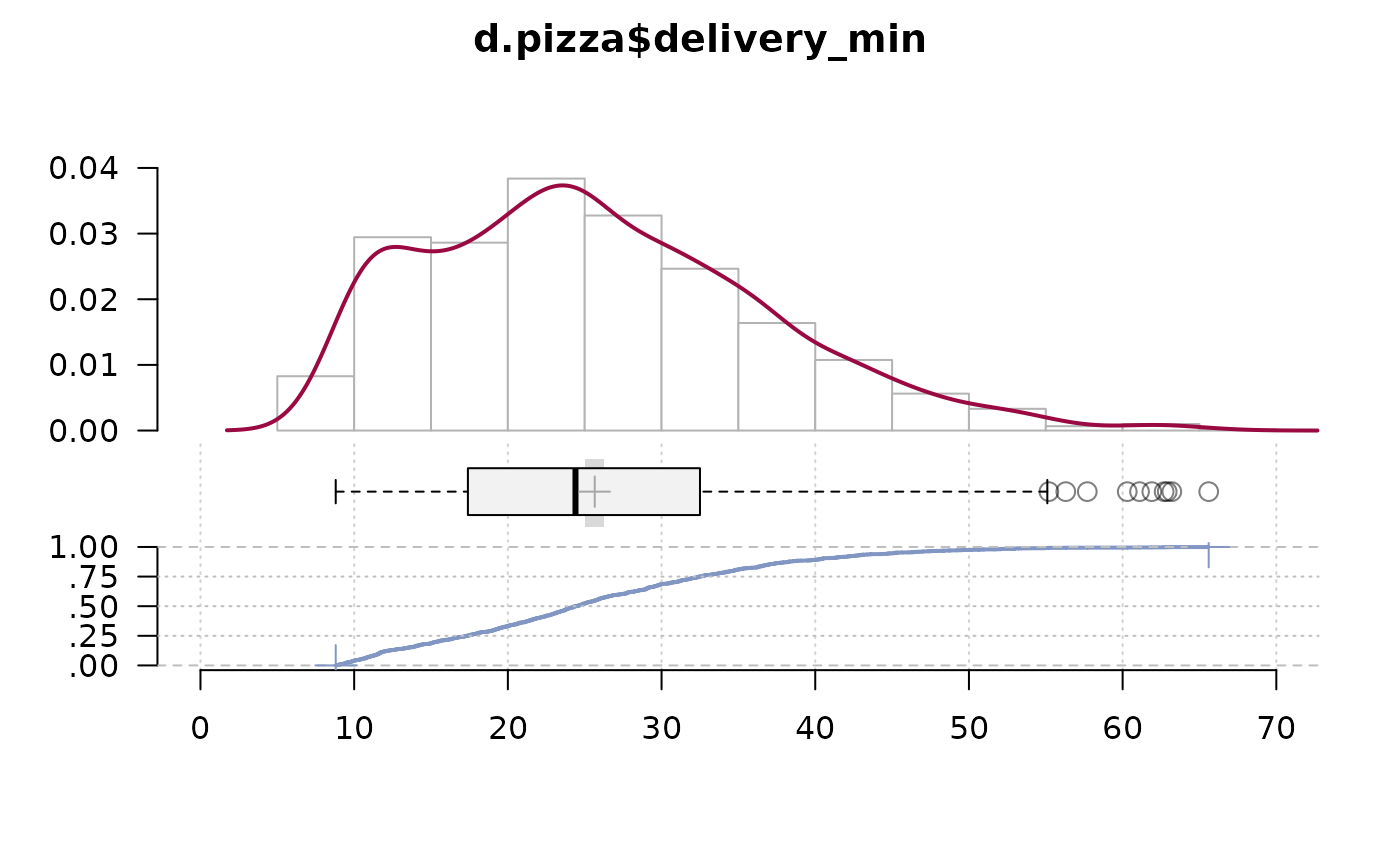
PlotFdist(x=d.pizza$delivery_min, na.rm=TRUE)
 # define additional arguments for hist, dens and boxplot
# do not display the mean and its CI on the boxplot
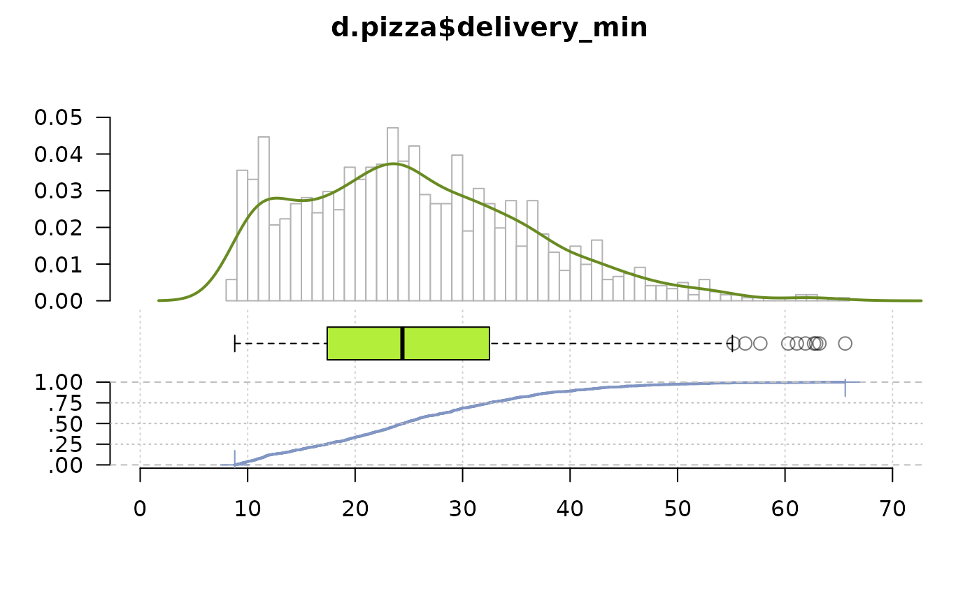
PlotFdist(d.pizza$delivery_min, args.hist=list(breaks=50),
args.dens=list(col="olivedrab4"), na.rm=TRUE,
args.boxplot=list(col="olivedrab2", pch.mean=NA, col.meanci=NA))
# define additional arguments for hist, dens and boxplot
# do not display the mean and its CI on the boxplot
PlotFdist(d.pizza$delivery_min, args.hist=list(breaks=50),
args.dens=list(col="olivedrab4"), na.rm=TRUE,
args.boxplot=list(col="olivedrab2", pch.mean=NA, col.meanci=NA))
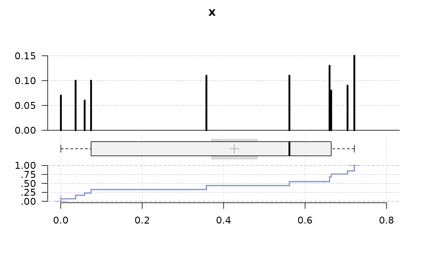
 # do a "h"-plot instead of a histogram for integers
x <- sample(runif(10), 100, replace = TRUE)
PlotFdist(x, args.hist=list(type="mass"))
# do a "h"-plot instead of a histogram for integers
x <- sample(runif(10), 100, replace = TRUE)
PlotFdist(x, args.hist=list(type="mass"))
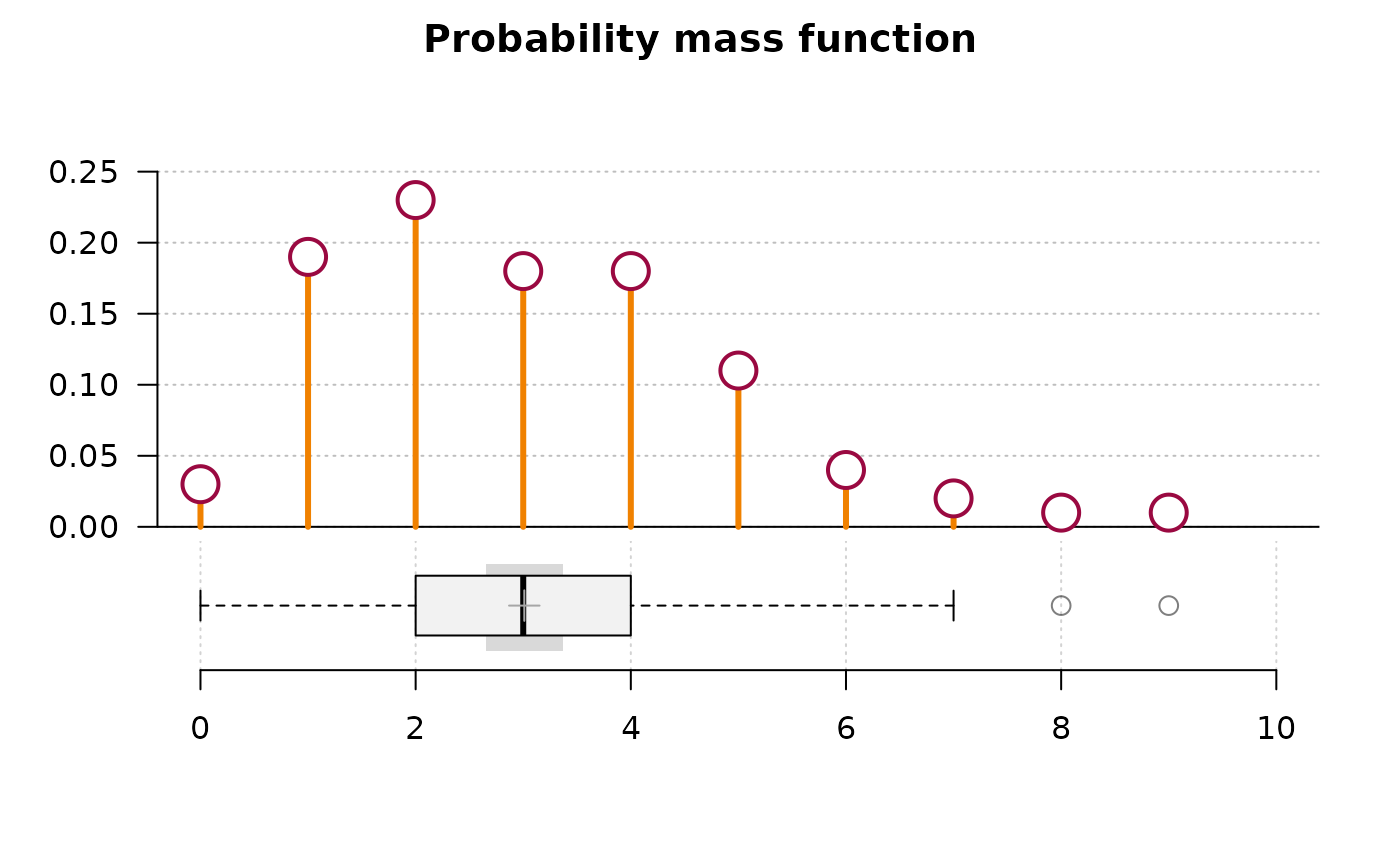
 pp <- rpois(n = 100, lambda = 3)
PlotFdist(pp, args.hist = list(type="mass", pch=21, col=DescTools::horange,
cex.pch=2.5, col.pch=DescTools::hred, lwd=3, bg.pch="white"),
args.boxplot = NULL, args.ecdf = NA, main="Probability mass function")
pp <- rpois(n = 100, lambda = 3)
PlotFdist(pp, args.hist = list(type="mass", pch=21, col=DescTools::horange,
cex.pch=2.5, col.pch=DescTools::hred, lwd=3, bg.pch="white"),
args.boxplot = NULL, args.ecdf = NA, main="Probability mass function")
 # special arguments for hist, density and ecdf
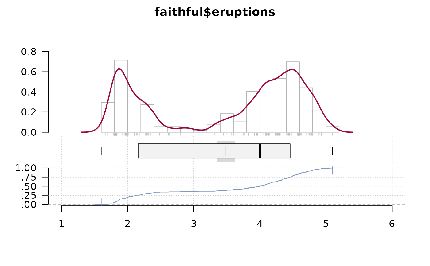
PlotFdist(x=faithful$eruptions,
args.hist=list(breaks=20), args.dens=list(bw=.1),
args.ecdf=list(cex=1.2, pch=16, lwd=1), args.rug=TRUE)
# special arguments for hist, density and ecdf
PlotFdist(x=faithful$eruptions,
args.hist=list(breaks=20), args.dens=list(bw=.1),
args.ecdf=list(cex=1.2, pch=16, lwd=1), args.rug=TRUE)
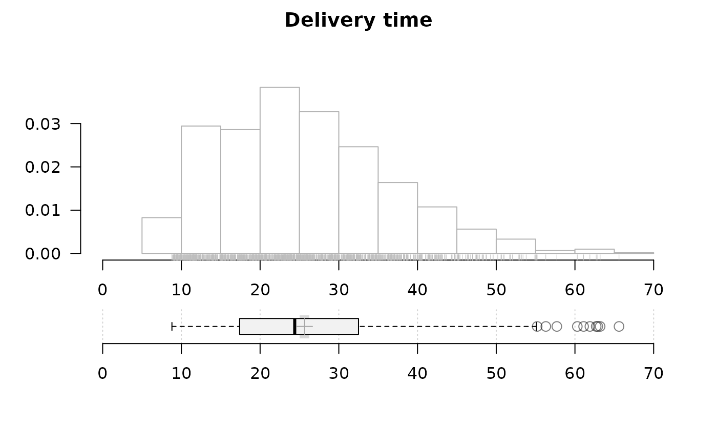
 # no density curve, no ecdf but add rug instead, make boxplot a bit higher
PlotFdist(x=d.pizza$delivery_min, na.rm=TRUE, args.dens=NA, args.ecdf=NA,
args.hist=list(xaxt="s"), # display x-axis on the histogram
args.rug=TRUE, heights=c(3, 2.5), pdist=2.5, main="Delivery time")
# no density curve, no ecdf but add rug instead, make boxplot a bit higher
PlotFdist(x=d.pizza$delivery_min, na.rm=TRUE, args.dens=NA, args.ecdf=NA,
args.hist=list(xaxt="s"), # display x-axis on the histogram
args.rug=TRUE, heights=c(3, 2.5), pdist=2.5, main="Delivery time")
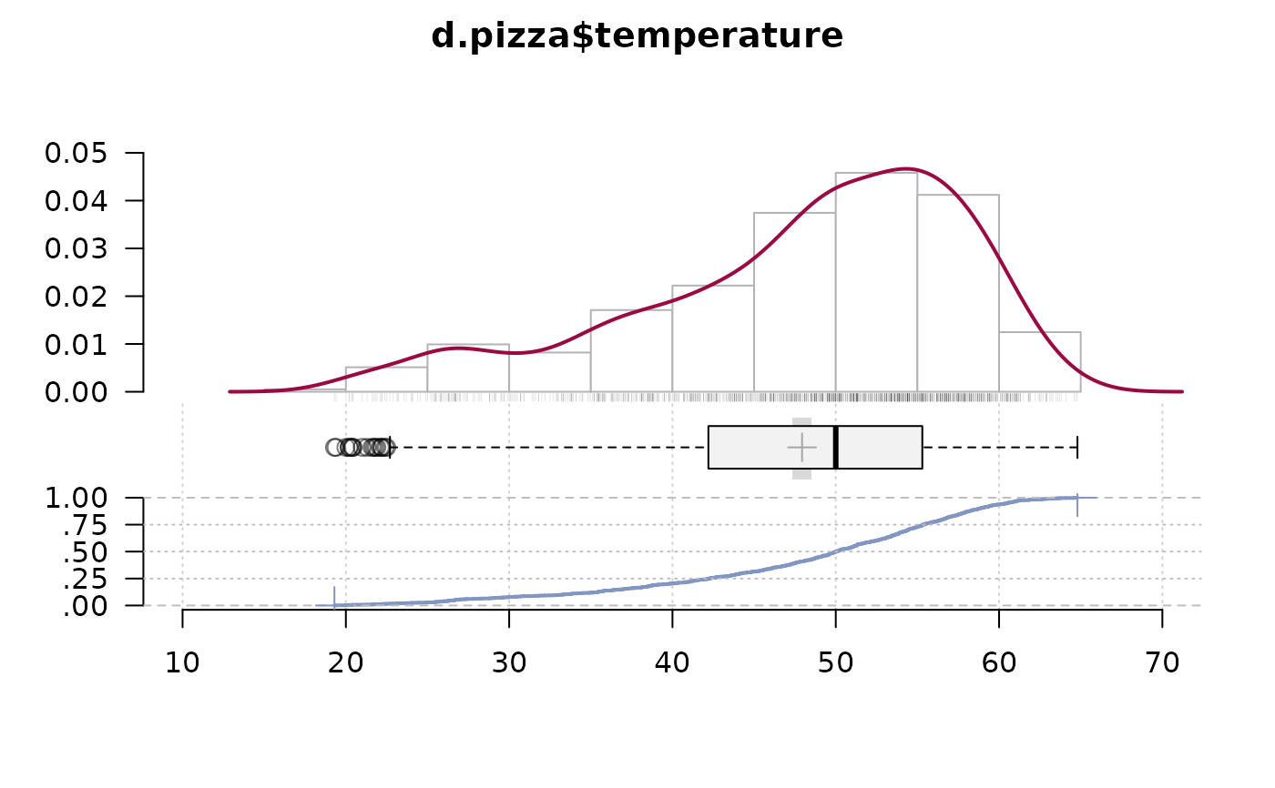
 # alpha channel on rug is cool, but takes its time for being drawn...
PlotFdist(x=d.pizza$temperature, args.rug=list(col=SetAlpha("black", 0.1)), na.rm=TRUE)
# alpha channel on rug is cool, but takes its time for being drawn...
PlotFdist(x=d.pizza$temperature, args.rug=list(col=SetAlpha("black", 0.1)), na.rm=TRUE)
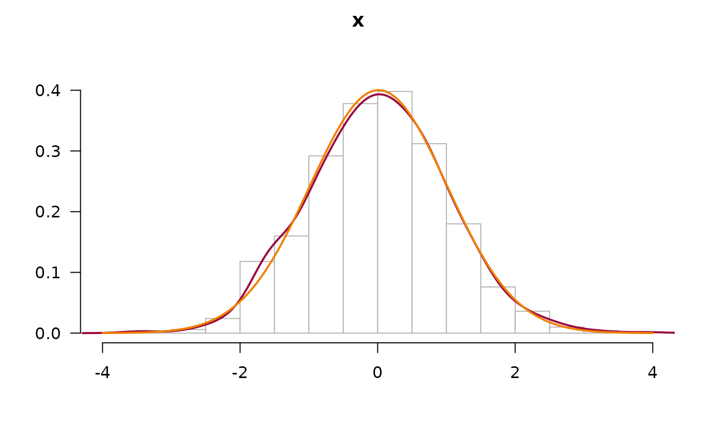
 # plot a normal density curve, but no boxplot nor ecdf
x <- rnorm(1000)
PlotFdist(x, args.curve = NULL, args.boxplot=NA, args.ecdf=NA)
# plot a normal density curve, but no boxplot nor ecdf
x <- rnorm(1000)
PlotFdist(x, args.curve = NULL, args.boxplot=NA, args.ecdf=NA)
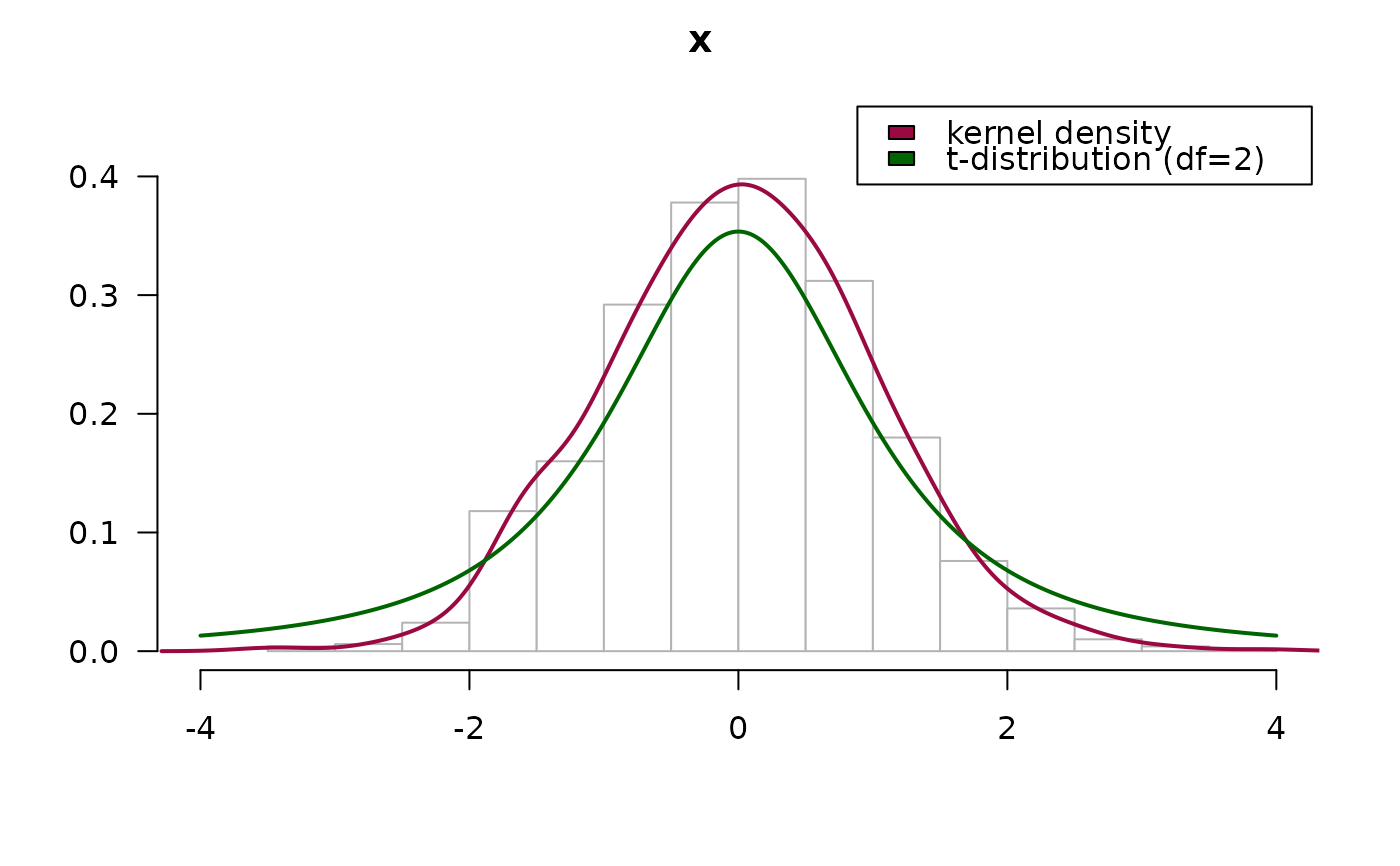
 # compare with a t-distribution
PlotFdist(x, args.curve = list(expr="dt(x, df=2)", col="darkgreen"),
args.boxplot=NA, args.ecdf=NA)
legend(x="topright", legend=c("kernel density", "t-distribution (df=2)"),
fill=c(getOption("col1", DescTools::hred), "darkgreen"), xpd=NA)
# compare with a t-distribution
PlotFdist(x, args.curve = list(expr="dt(x, df=2)", col="darkgreen"),
args.boxplot=NA, args.ecdf=NA)
legend(x="topright", legend=c("kernel density", "t-distribution (df=2)"),
fill=c(getOption("col1", DescTools::hred), "darkgreen"), xpd=NA)
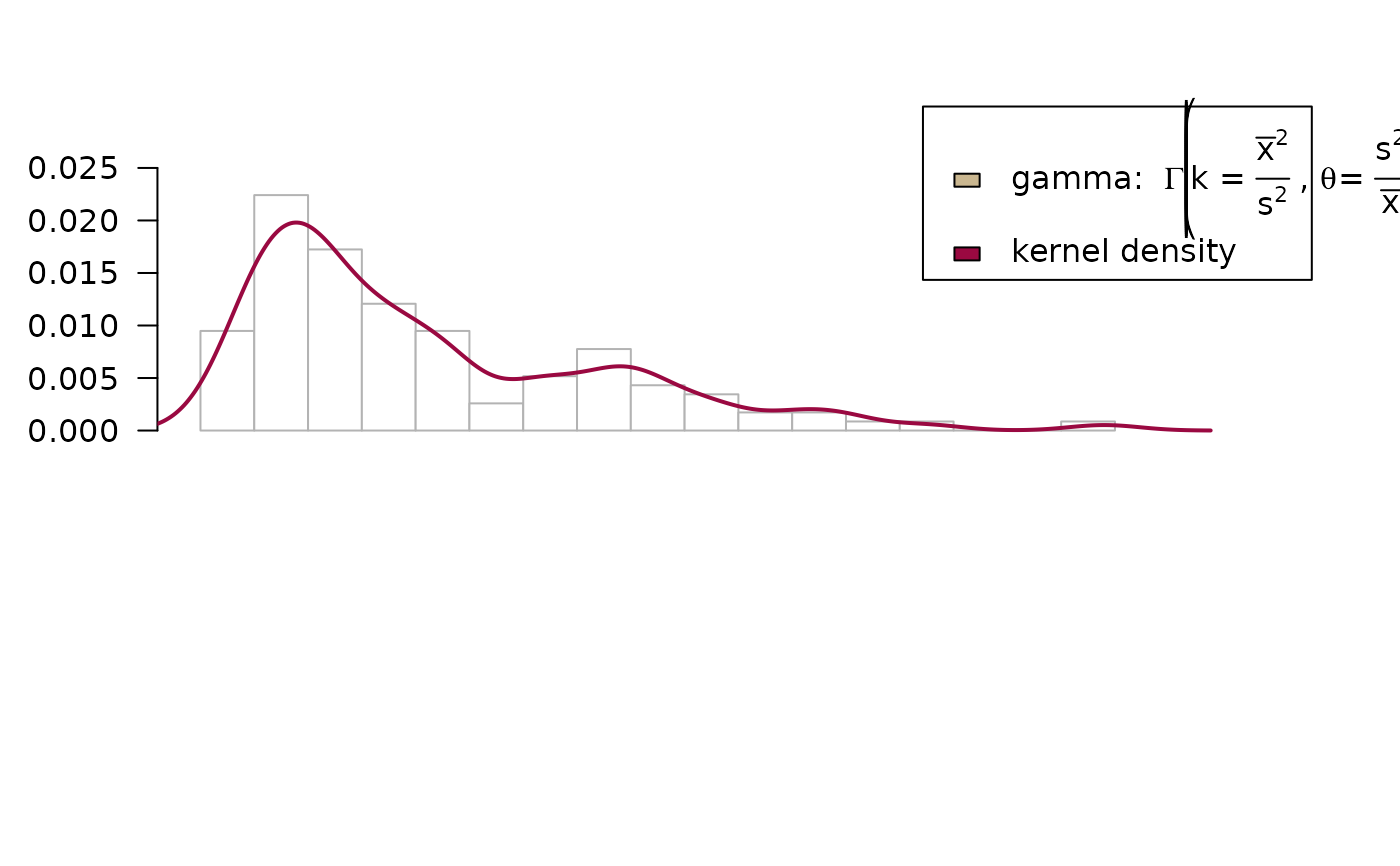
 # add a gamma distribution curve to both, histogram and ecdf
ozone <- airquality$Ozone; m <- mean(ozone, na.rm = TRUE); v <- var(ozone, na.rm = TRUE)
PlotFdist(ozone, args.hist = list(breaks=15),
args.curve = list(expr="dgamma(x, shape = m^2/v, scale = v/m)", col=DescTools::hecru),
args.curve.ecdf = list(expr="pgamma(x, shape = m^2/v, scale = v/m)", col=DescTools::hecru),
na.rm = TRUE, main = "Airquality - Ozone")
#> Error in eval(expr, envir = ll, enclos = parent.frame()): object 'm' not found
legend(x="topright", xpd=NA,
legend=c(expression(plain("gamma: ") * Gamma * " " * bgroup("(", k * " = " *
over(bar(x)^2, s^2) * " , " * theta * plain(" = ") * over(s^2, bar(x)), ")") ),
"kernel density"),
fill=c(DescTools::hecru, getOption("col1", DescTools::hred)), text.width = 0.25)
# add a gamma distribution curve to both, histogram and ecdf
ozone <- airquality$Ozone; m <- mean(ozone, na.rm = TRUE); v <- var(ozone, na.rm = TRUE)
PlotFdist(ozone, args.hist = list(breaks=15),
args.curve = list(expr="dgamma(x, shape = m^2/v, scale = v/m)", col=DescTools::hecru),
args.curve.ecdf = list(expr="pgamma(x, shape = m^2/v, scale = v/m)", col=DescTools::hecru),
na.rm = TRUE, main = "Airquality - Ozone")
#> Error in eval(expr, envir = ll, enclos = parent.frame()): object 'm' not found
legend(x="topright", xpd=NA,
legend=c(expression(plain("gamma: ") * Gamma * " " * bgroup("(", k * " = " *
over(bar(x)^2, s^2) * " , " * theta * plain(" = ") * over(s^2, bar(x)), ")") ),
"kernel density"),
fill=c(DescTools::hecru, getOption("col1", DescTools::hred)), text.width = 0.25)