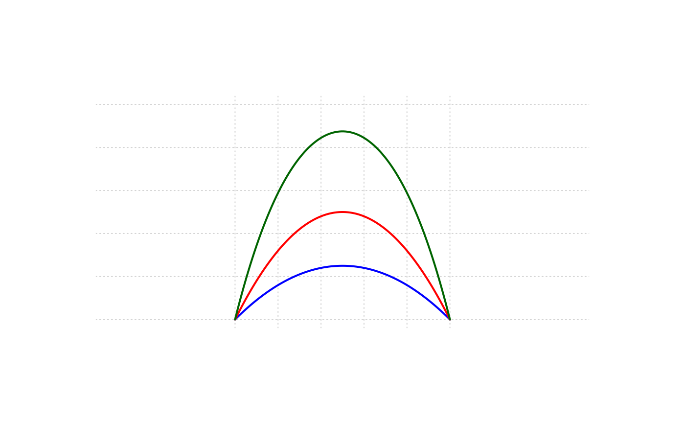
Draw a Bezier Curve
DrawBezier.RdDraw a Bezier curve.
Arguments
- x, y
a vector of xy-coordinates to define the Bezier curve. Should at least contain 3 points.
- nv
number of vertices to draw the curve.
- col
color(s) for the curve. Default is
par("fg").- lty
line type for borders and shading; defaults to
"solid".- lwd
line width for borders and shading.
- plot
logical. If
TRUEthe structure will be plotted. IfFALSEonly the xy-points are calculated and returned. Use this if you want to combine several geometric structures to a single polygon.
Details
Bezier curves appear in such areas as mechanical computer aided design (CAD). They are named after P. Bezier, who used a closely related representation in Renault's UNISURF CAD system in the early 1960s (similar, unpublished, work was done by P. de Casteljau at Citroen in the late 1950s and early 1960s). The 1970s and 1980s saw a flowering of interest in Bezier curves, with many CAD systems using them, and many important developments in their theory. The usefulness of Bezier curves resides in their many geometric and analytical properties. There are elegant and efficient algorithms for evaluation, differentiation, subdivision of the curves, and conversion to other useful representations. (See: Farin, 1993)
Value
DrawBezier invisibly returns a list of the calculated coordinates for all shapes.
References
G. Farin (1993) Curves and surfaces for computer aided geometric design. A practical guide, Acad. Press