Collapse Levels of a Table
CollapseTable.RdCollapse (or re-label) variables in a
a contingency table or ftable object by re-assigning levels of the table variables.
CollapseTable(x, ...)Arguments
Details
Each of the ... arguments must be of the form
variable = levels, where variable is the name of one of the table
dimensions, and levels is a character or numeric vector of length equal
to the corresponding dimension of the table. Missing argument names are allowed and will be interpreted in the order of the dimensions of the table.
Value
A table object (even if the input was an ftable), representing the original table with
one or more of its factors collapsed or rearranged into other levels.
See also
margin.table "collapses" a table in a different way, by
summing over table dimensions.
Examples
# create some sample data in table form
sex <- c("Male", "Female")
age <- letters[1:6]
education <- c("low", 'med', 'high')
data <- expand.grid(sex=sex, age=age, education=education)
counts <- rpois(36, 100)
data <- cbind(data, counts)
t1 <- xtabs(counts ~ sex + age + education, data=data)
Desc(t1)
#> ──────────────────────────────────────────────────────────────────────────────
#> t1 (xtabs, table)
#>
#> Summary:
#> n: 3'706, 3-dim table: 2 x 6 x 3
#>
#> Chi-squared test for independence of all factors:
#> X-squared = 17.972, df = 27, p-value = 0.9044
#>
#> education low med high Sum
#> sex age
#> Male a 105 103 107 315
#> b 98 113 109 320
#> c 95 114 86 295
#> d 85 105 97 287
#> e 107 105 112 324
#> f 112 110 106 328
#> Female a 111 107 109 327
#> b 102 106 95 303
#> c 86 102 87 275
#> d 100 107 84 291
#> e 84 103 107 294
#> f 127 115 105 347
#> Sum a 216 210 216 642
#> b 200 219 204 623
#> c 181 216 173 570
#> d 185 212 181 578
#> e 191 208 219 618
#> f 239 225 211 675
#>
 ## age a b c d e f
## sex education
## Male low 119 101 109 85 99 93
## med 94 98 103 108 84 84
## high 81 88 96 110 100 92
## Female low 107 104 95 86 103 96
## med 104 98 94 95 110 106
## high 93 85 90 109 99 86
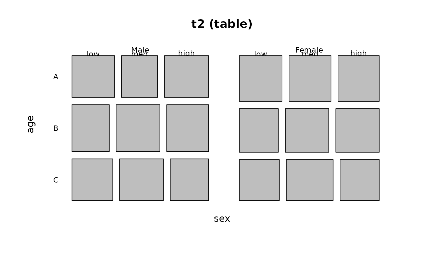
# collapse age to 3 levels
t2 <- CollapseTable(t1, age=c("A", "A", "B", "B", "C", "C"))
Desc(t2)
#> ──────────────────────────────────────────────────────────────────────────────
#> t2 (table)
#>
#> Summary:
#> n: 3'706, 3-dim table: 2 x 3 x 3
#>
#> Chi-squared test for independence of all factors:
#> X-squared = 6.038, df = 12, p-value = 0.9142
#>
#> education low med high Sum
#> sex age
#> Male A 203 216 216 635
#> B 180 219 183 582
#> C 219 215 218 652
#> Female A 213 213 204 630
#> B 186 209 171 566
#> C 211 218 212 641
#> Sum A 416 429 420 1265
#> B 366 428 354 1148
#> C 430 433 430 1293
#>
## age a b c d e f
## sex education
## Male low 119 101 109 85 99 93
## med 94 98 103 108 84 84
## high 81 88 96 110 100 92
## Female low 107 104 95 86 103 96
## med 104 98 94 95 110 106
## high 93 85 90 109 99 86
# collapse age to 3 levels
t2 <- CollapseTable(t1, age=c("A", "A", "B", "B", "C", "C"))
Desc(t2)
#> ──────────────────────────────────────────────────────────────────────────────
#> t2 (table)
#>
#> Summary:
#> n: 3'706, 3-dim table: 2 x 3 x 3
#>
#> Chi-squared test for independence of all factors:
#> X-squared = 6.038, df = 12, p-value = 0.9142
#>
#> education low med high Sum
#> sex age
#> Male A 203 216 216 635
#> B 180 219 183 582
#> C 219 215 218 652
#> Female A 213 213 204 630
#> B 186 209 171 566
#> C 211 218 212 641
#> Sum A 416 429 420 1265
#> B 366 428 354 1148
#> C 430 433 430 1293
#>
 ## age A B C
## sex education
## Male low 220 194 192
## med 192 211 168
## high 169 206 192
## Female low 211 181 199
## med 202 189 216
## high 178 199 185
# collapse age to 3 levels and pool education: "low" and "med" to "low"
t3 <- CollapseTable(t1, age=c("A", "A", "B", "B", "C", "C"),
education=c("low", "low", "high"))
Desc(t3)
#> ──────────────────────────────────────────────────────────────────────────────
#> t3 (table)
#>
#> Summary:
#> n: 3'706, 3-dim table: 2 x 3 x 2
#>
#> Chi-squared test for independence of all factors:
#> X-squared = 2.724, df = 7, p-value = 0.9093
#>
#> education low high Sum
#> sex age
#> Male A 419 216 635
#> B 399 183 582
#> C 434 218 652
#> Female A 426 204 630
#> B 395 171 566
#> C 429 212 641
#> Sum A 845 420 1265
#> B 794 354 1148
#> C 863 430 1293
#>
## age A B C
## sex education
## Male low 220 194 192
## med 192 211 168
## high 169 206 192
## Female low 211 181 199
## med 202 189 216
## high 178 199 185
# collapse age to 3 levels and pool education: "low" and "med" to "low"
t3 <- CollapseTable(t1, age=c("A", "A", "B", "B", "C", "C"),
education=c("low", "low", "high"))
Desc(t3)
#> ──────────────────────────────────────────────────────────────────────────────
#> t3 (table)
#>
#> Summary:
#> n: 3'706, 3-dim table: 2 x 3 x 2
#>
#> Chi-squared test for independence of all factors:
#> X-squared = 2.724, df = 7, p-value = 0.9093
#>
#> education low high Sum
#> sex age
#> Male A 419 216 635
#> B 399 183 582
#> C 434 218 652
#> Female A 426 204 630
#> B 395 171 566
#> C 429 212 641
#> Sum A 845 420 1265
#> B 794 354 1148
#> C 863 430 1293
#>
 ## age A B C
## sex education
## Male low 412 405 360
## high 169 206 192
## Female low 413 370 415
## high 178 199 185
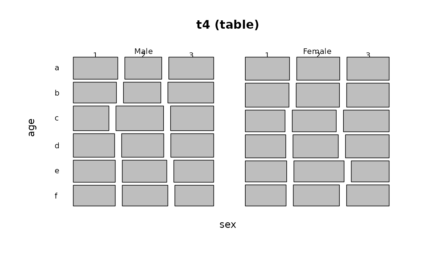
# change labels for levels of education to 1:3
t4 <- CollapseTable(t1, education=1:3)
Desc(t4)
#> ──────────────────────────────────────────────────────────────────────────────
#> t4 (table)
#>
#> Summary:
#> n: 3'706, 3-dim table: 2 x 6 x 3
#>
#> Chi-squared test for independence of all factors:
#> X-squared = 17.972, df = 27, p-value = 0.9044
#>
#> education 1 2 3 Sum
#> sex age
#> Male a 105 103 107 315
#> b 98 113 109 320
#> c 95 114 86 295
#> d 85 105 97 287
#> e 107 105 112 324
#> f 112 110 106 328
#> Female a 111 107 109 327
#> b 102 106 95 303
#> c 86 102 87 275
#> d 100 107 84 291
#> e 84 103 107 294
#> f 127 115 105 347
#> Sum a 216 210 216 642
#> b 200 219 204 623
#> c 181 216 173 570
#> d 185 212 181 578
#> e 191 208 219 618
#> f 239 225 211 675
#>
## age A B C
## sex education
## Male low 412 405 360
## high 169 206 192
## Female low 413 370 415
## high 178 199 185
# change labels for levels of education to 1:3
t4 <- CollapseTable(t1, education=1:3)
Desc(t4)
#> ──────────────────────────────────────────────────────────────────────────────
#> t4 (table)
#>
#> Summary:
#> n: 3'706, 3-dim table: 2 x 6 x 3
#>
#> Chi-squared test for independence of all factors:
#> X-squared = 17.972, df = 27, p-value = 0.9044
#>
#> education 1 2 3 Sum
#> sex age
#> Male a 105 103 107 315
#> b 98 113 109 320
#> c 95 114 86 295
#> d 85 105 97 287
#> e 107 105 112 324
#> f 112 110 106 328
#> Female a 111 107 109 327
#> b 102 106 95 303
#> c 86 102 87 275
#> d 100 107 84 291
#> e 84 103 107 294
#> f 127 115 105 347
#> Sum a 216 210 216 642
#> b 200 219 204 623
#> c 181 216 173 570
#> d 185 212 181 578
#> e 191 208 219 618
#> f 239 225 211 675
#>
 ## age a b c d e f
## sex education
## Male 1 119 101 109 85 99 93
## 2 94 98 103 108 84 84
## 3 81 88 96 110 100 92
## Female 1 107 104 95 86 103 96
## 2 104 98 94 95 110 106
## 3 93 85 90 109 99 86
## age a b c d e f
## sex education
## Male 1 119 101 109 85 99 93
## 2 94 98 103 108 84 84
## 3 81 88 96 110 100 92
## Female 1 107 104 95 86 103 96
## 2 104 98 94 95 110 106
## 3 93 85 90 109 99 86